Why Autoencoders Matter: Deep Learning’s Most Underrated Techniques

Discover why autoencoders are deep learning’s most underrated technique in 2025. Learn how these powerful neural networks enable anomaly detection, data compression, and feature learning with practical Python implementations

Introduction: The Silent Workhorse of Modern AI

In the dazzling world of 2025’s artificial intelligence, dominated by headline-grabbing large language models and generative video systems, it’s easy for foundational techniques to be overlooked. Yet, powering many of these advancements and solving critical, unglamorous problems is one of deep learning’s most versatile and underrated architectures: the autoencoder.

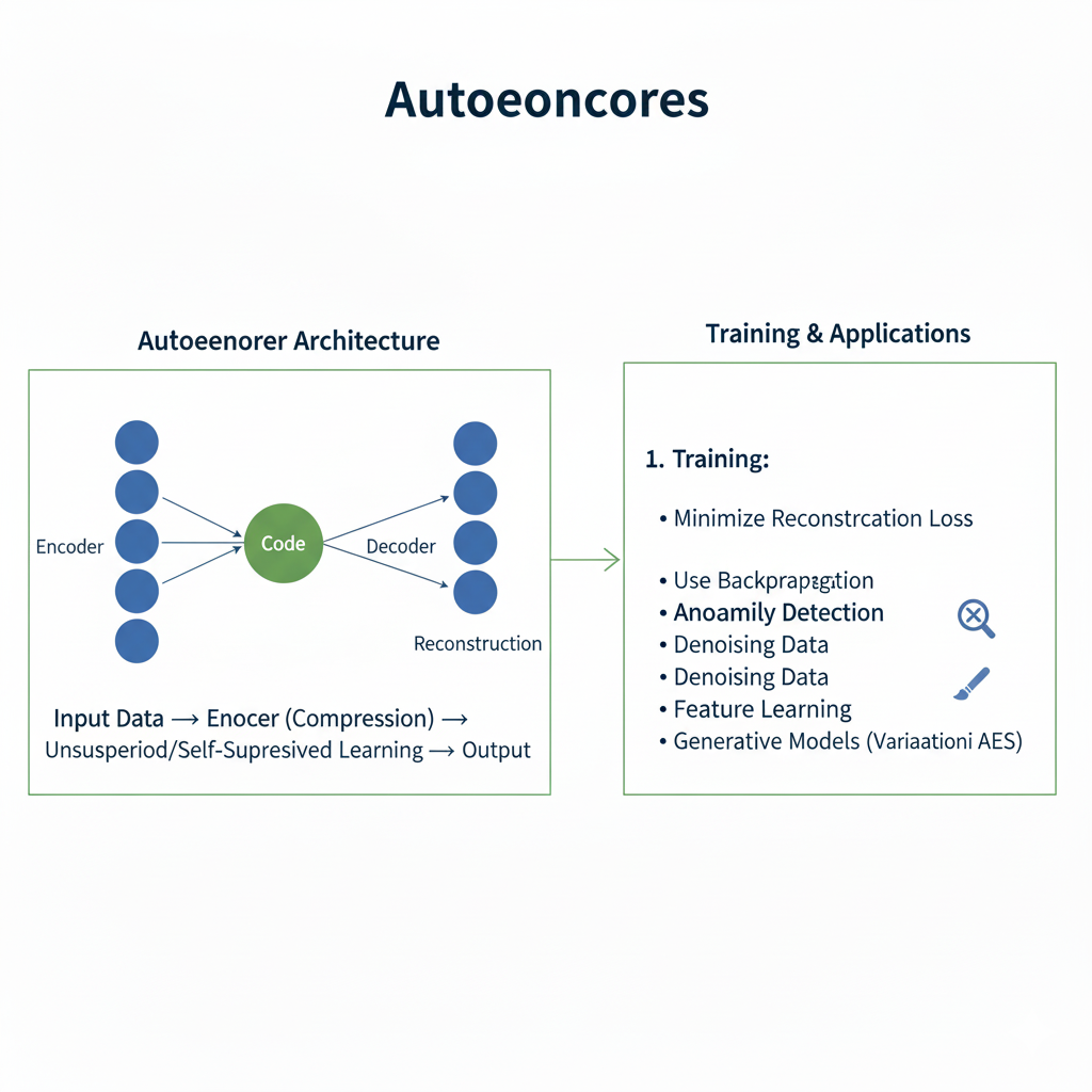
An autoencoder is a type of neural network designed to learn efficient representations of data, typically for the purpose of dimensionality reduction or feature learning. In its simplest form, it is trained to copy its input to its output. This may sound trivial, but the magic lies in the constraint: it must first compress the data into a lower-dimensional latent space, a bottleneck, before reconstructing it. By learning to reconstruct the input from this compressed representation, the network is forced to capture the most salient features of the data.

Far from being a relic of deep learning’s past, the autoencoder has evolved. In 2025, it is not a single algorithm but a family of powerful, specialized tools essential for data compression, anomaly detection, and as a foundational component in generative AI. This article will explore why this unassuming architecture remains a critical piece of the modern AI toolkit, detailing its core principles, its advanced variants, and its practical applications that are more relevant today than ever before.

Part 1: The Foundational Principle – Learning to Represent Data

At its heart, the autoencoder is built on a beautifully simple concept: learning the identity function through an information bottleneck. This forced compression is what drives it to discover meaningful patterns.

1.1 The Architectural Blueprint: Encoder, Bottleneck, Decoder

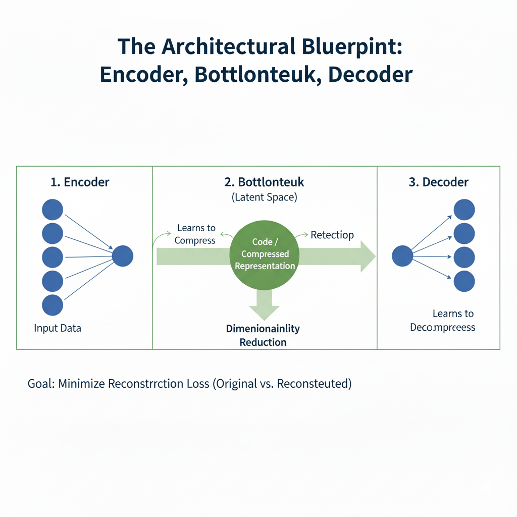
Every autoencoder consists of three core components:

1. Encoder: This is the part of the network that compresses the input into a latent-space representation. It learns to map high-dimensional input data to a lower-dimensional code. For an image, this might involve reducing a 784-pixel MNIST digit down to a vector of just 32 numbers that capture its essence—its shape, slant, and thickness.
   • Operation: z = encoder(x)
2. Bottleneck (Latent Space): This layer contains the compressed knowledge of the input data. It is the most crucial part of the network. Its limited capacity creates an “information bottleneck,” forcing the encoder to learn a smart, compressed representation and preventing the network from simply learning to copy the input.
   • Representation: The code z, a dense vector of features.
3. Decoder: This part of the network aims to reconstruct the input data from the latent space representation. It mirrors the encoder’s architecture, progressively upsampling the data back to its original dimensions.
   • Operation: x' = decoder(z)

The network is trained end-to-end by minimizing a reconstruction loss, such as Mean Squared Error (MSE) or Binary Cross-Entropy, which measures the difference between the original input x and the reconstructed output x'.

1.2 The “Why”: What Does This Achieve?

By solving this reconstruction task, the autoencoder learns a powerful, non-linear form of dimensionality reduction. It’s often described as a more powerful, flexible successor to older techniques like Principal Component Analysis (PCA). However, its utility goes far beyond compression:

• Feature Learning: The latent representation z often contains a distilled version of the data’s most important features. This representation can be used as input for other machine learning models, often leading to better performance than using the raw data.
• Denoising: By training the network to reconstruct clean data from noisy inputs, it learns to filter out noise and corruptions.
• Anomaly Detection: A well-trained autoencoder will be very good at reconstructing “normal” data it has seen before but poor at reconstructing anomalous or novel data. This high reconstruction error can be used to flag outliers.

Part 2: A Practical Walkthrough – Building a Modern Autoencoder in 2025

Let’s move from theory to practice by building a convolutional autoencoder for image denoising, implemented with 2025’s best practices in TensorFlow/Keras.

python

import tensorflow as tf
from tensorflow.keras import layers, models, losses, callbacks
import numpy as np
import matplotlib.pyplot as plt

# Load and preprocess the MNIST dataset
(x_train, _), (x_test, _) = tf.keras.datasets.mnist.load_data() # We don't need the labels

# Normalize and reshape the images
x_train = x_train.astype('float32') / 255.
x_test = x_test.astype('float32') / 255.
x_train = np.reshape(x_train, (len(x_train), 28, 28, 1))
x_test = np.reshape(x_test, (len(x_test), 28, 28, 1))

# Add synthetic noise to the images
def add_noise(images, noise_factor=0.5):
    noisy = images + noise_factor * np.random.normal(loc=0.0, scale=1.0, size=images.shape)
    # Clip the images to be between 0 and 1
    noisy = np.clip(noisy, 0., 1.)
    return noisy

# Create noisy versions of the training and test sets
x_train_noisy = add_noise(x_train)
x_test_noisy = add_noise(x_test)

print(f"Training data shape: {x_train.shape}")
print(f"Noisy training data shape: {x_train_noisy.shape}")

def create_convolutional_autoencoder(input_shape=(28, 28, 1)):
    """
    Creates a convolutional denoising autoencoder with modern practices.
    """
    # Input layer
    input_img = layers.Input(shape=input_shape)
    
    # --- Encoder ---
    x = layers.Conv2D(32, (3, 3), activation='swish', padding='same')(input_img)
    x = layers.BatchNormalization()(x)
    x = layers.MaxPooling2D((2, 2), padding='same')(x) # 14x14
    
    x = layers.Conv2D(32, (3, 3), activation='swish', padding='same')(x)
    x = layers.BatchNormalization()(x)
    encoded = layers.MaxPooling2D((2, 2), padding='same')(x) # 7x7x32 - This is the bottleneck!
    
    # --- Decoder ---
    x = layers.Conv2D(32, (3, 3), activation='swish', padding='same')(encoded)
    x = layers.BatchNormalization()(x)
    x = layers.UpSampling2D((2, 2))(x) # 14x14
    
    x = layers.Conv2D(32, (3, 3), activation='swish', padding='same')(x)
    x = layers.BatchNormalization()(x)
    x = layers.UpSampling2D((2, 2))(x) # 28x28
    
    # Output layer (single filter with sigmoid activation)
    decoded = layers.Conv2D(1, (3, 3), activation='sigmoid', padding='same')(x)
    
    # Create the autoencoder model
    autoencoder = models.Model(input_img, decoded)
    return autoencoder

# Create and compile the model
autoencoder = create_convolutional_autoencoder()
autoencoder.compile(optimizer='adamw', loss='binary_crossentropy')

# Display the architecture
autoencoder.summary()

# Define callbacks for better training
training_callbacks = [
    callbacks.EarlyStopping(monitor='val_loss', patience=10, restore_best_weights=True),
    callbacks.ReduceLROnPlateau(monitor='val_loss', factor=0.5, patience=5, verbose=1)
]

# Train the model to reconstruct clean images from noisy ones
print("Training the denoising autoencoder...")
history = autoencoder.fit(
    x_train_noisy, x_train, # Input: Noisy, Target: Clean
    epochs=50,
    batch_size=128,
    shuffle=True,
    validation_data=(x_test_noisy, x_test),
    callbacks=training_callbacks,
    verbose=1
)

# Evaluate the model
test_loss = autoencoder.evaluate(x_test_noisy, x_test, verbose=0)
print(f"Final Test Loss: {test_loss:.4f}")

# Visualize the denoising results
def visualize_results(original, noisy, denoised, num_images=5):
    plt.figure(figsize=(10, 6))
    
    for i in range(num_images):
        # Display original images
        ax = plt.subplot(3, num_images, i + 1)
        plt.imshow(original[i].reshape(28, 28), cmap='gray')
        plt.title("Original")
        plt.axis('off')
        
        # Display noisy images
        ax = plt.subplot(3, num_images, i + 1 + num_images)
        plt.imshow(noisy[i].reshape(28, 28), cmap='gray')
        plt.title("Noisy Input")
        plt.axis('off')
        
        # Display reconstructed images
        ax = plt.subplot(3, num_images, i + 1 + 2 * num_images)
        plt.imshow(denoised[i].reshape(28, 28), cmap='gray')
        plt.title("Denoised")
        plt.axis('off')
    
    plt.tight_layout()
    plt.show()

# Generate denoised images
denoised_imgs = autoencoder.predict(x_test_noisy[:5])
visualize_results(x_test[:5], x_test_noisy[:5], denoised_imgs)

Key 2025 Best Practices Demonstrated:

• Swish Activation: A modern activation function that often outperforms ReLU.
• Batch Normalization: Used after convolutional layers to stabilize and accelerate training.
• AdamW Optimizer: The modern standard with decoupled weight decay.
• Advanced Callbacks: Automated learning rate reduction and early stopping.
• Convolutional Architecture: Essential for capturing spatial hierarchies in image data.

Part 3: The Evolutionary Tree – Key Variants and Their Superpowers

The basic autoencoder is a starting point. Its true power is revealed in its specialized variants, each designed to solve specific problems.

3.1 Denoising Autoencoder (DAE)

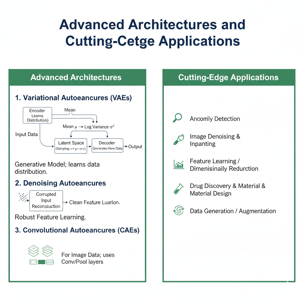
As demonstrated above, this variant is trained to reconstruct clean data from a corrupted or noisy input. By learning to remove noise, it is forced to understand the true underlying structure of the data, leading to more robust feature learning.

3.2 Variational Autoencoder (VAE): The Bridge to Generative AI

The Variational Autoencoder is a monumental leap. Instead of learning a fixed compression, it learns the parameters of a probability distribution (typically a Gaussian) for the latent space. During training, it samples from this distribution to generate the decoder’s input.

• How it works: The encoder outputs two vectors: a mean (μ) and a standard deviation (σ). It then samples a latent vector z using the “reparameterization trick”: z = μ + σ * ε, where ε is random noise.
• The Loss Function: The VAE loss has two parts:
  1. Reconstruction Loss: The familiar difference between input and output.
  2. KL Divergence: A regularization term that forces the learned latent distribution to be close to a standard normal distribution. This ensures the latent space is continuous and structured.

This structured, probabilistic latent space is what makes VAEs powerful generative models. You can sample a random vector from the latent distribution and decode it into a new, coherent data sample.

python

# Simplified VAE implementation
class Sampling(layers.Layer):
    """Uses (z_mean, z_log_var) to sample z, the vector encoding a digit."""
    def call(self, inputs):
        z_mean, z_log_var = inputs
        batch = tf.shape(z_mean)[0]
        dim = tf.shape(z_mean)[1]
        epsilon = tf.keras.backend.random_normal(shape=(batch, dim))
        return z_mean + tf.exp(0.5 * z_log_var) * epsilon

def create_variational_autoencoder(latent_dim=2):
    # Encoder
    encoder_inputs = layers.Input(shape=(28, 28, 1))
    x = layers.Conv2D(32, 3, activation="swish", strides=2, padding="same")(encoder_inputs)
    x = layers.Conv2D(64, 3, activation="swish", strides=2, padding="same")(x)
    x = layers.Flatten()(x)
    x = layers.Dense(16, activation="swish")(x)
    z_mean = layers.Dense(latent_dim, name="z_mean")(x)
    z_log_var = layers.Dense(latent_dim, name="z_log_var")(x)
    z = Sampling()([z_mean, z_log_var])
    encoder = models.Model(encoder_inputs, [z_mean, z_log_var, z], name="encoder")

    # Decoder
    latent_inputs = layers.Input(shape=(latent_dim,))
    x = layers.Dense(7 * 7 * 64, activation="swish")(latent_inputs)
    x = layers.Reshape((7, 7, 64))(x)
    x = layers.Conv2DTranspose(64, 3, activation="swish", strides=2, padding="same")(x)
    x = layers.Conv2DTranspose(32, 3, activation="swish", strides=2, padding="same")(x)
    decoder_outputs = layers.Conv2DTranspose(1, 3, activation="sigmoid", padding="same")(x)
    decoder = models.Model(latent_inputs, decoder_outputs, name="decoder")

    # VAE Model
    outputs = decoder(encoder(encoder_inputs)[2])
    vae = models.Model(encoder_inputs, outputs, name="vae")

    # Add KL divergence loss
    kl_loss = -0.5 * tf.reduce_mean(z_log_var - tf.square(z_mean) - tf.exp(z_log_var) + 1)
    vae.add_loss(kl_loss)
    vae.compile(optimizer="adamw")
    return vae, encoder, decoder

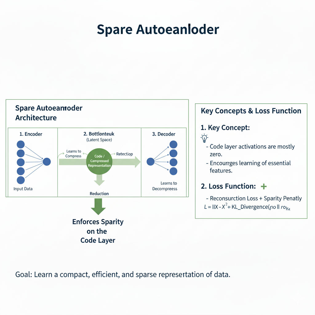
3.3 Sparse Autoencoder

This variant adds a sparsity constraint on the latent code, forcing the model to activate only a small number of neurons for any given input. This leads to the discovery of more independent, interpretable features, much like how individual neurons in the brain might respond to specific stimuli.

Part 4: The 2025 Application Landscape – Where Autoencoders Truly Shine

In the modern AI ecosystem, the autoencoder is not a competitor to large foundational models but a crucial complementary technology. Its applications are more critical than ever.

4.1 Anomaly Detection in High-Stakes Environments

In sectors like finance, healthcare, and cybersecurity, finding rare, abnormal events is paramount. An autoencoder trained exclusively on “normal” data becomes a highly sensitive anomaly detector.

• Process: After training on normal data, the model’s reconstruction error is calculated on new data points. A high error indicates the data point is anomalous and unlike anything seen during training.
• Real-World Example: Monitoring MRI scans for rare pathologies, detecting fraudulent financial transactions in real-time, or identifying novel cyber-attack patterns in network traffic.

python

def create_anomaly_detector(normal_data, contamination=0.1):
    """Creates an autoencoder-based anomaly detection system."""
    autoencoder = create_convolutional_autoencoder()
    autoencoder.compile(optimizer='adamw', loss='mse')
    
    # Train only on normal data
    autoencoder.fit(normal_data, normal_data, epochs=100, batch_size=128, verbose=0)
    
    # Calculate reconstruction error on training data
    reconstructions = autoencoder.predict(normal_data)
    train_loss = np.mean(np.square(normal_data - reconstructions), axis=(1,2,3))
    
    # Set threshold based on contamination rate
    threshold = np.percentile(train_loss, 100 * (1 - contamination))
    
    return autoencoder, threshold

def detect_anomalies(model, threshold, new_data):
    """Detect anomalies in new data."""
    reconstructions = model.predict(new_data)
    loss = np.mean(np.square(new_data - reconstructions), axis=(1,2,3))
    return loss > threshold, loss

4.2 Data Compression and Efficient Representation Learning

With the explosion of data in 2025, efficient storage and transmission are key. Autoencoders provide a form of “semantic compression,” where the compressed representation retains the most meaningful information, which is often more useful than generic compression like JPEG.

• Use Case: Compressing medical images for telemedicine while preserving diagnostically relevant features, or reducing the dimensionality of complex sensor data from industrial IoT devices for more efficient processing.

4.3 Feature Learning and Transfer Learning

The encoder of a pre-trained autoencoder can be used as a powerful, generic feature extractor. The features learned in the latent space are often more transferable and robust than those learned through supervised learning, as they are not tied to a specific classification task.

python

# Using a pre-trained autoencoder as a feature extractor
pretrained_encoder = create_convolutional_autoencoder().encoder

# Freeze the encoder layers
for layer in pretrained_encoder.layers:
    layer.trainable = False

# Build a classifier on top of the encoded features
classifier_input = layers.Input(shape=pretrained_encoder.output.shape[1:])
x = layers.GlobalAveragePooling2D()(classifier_input)
x = layers.Dense(128, activation='swish')(x)
classifier_output = layers.Dense(10, activation='softmax')(x) # For 10-class classification

classifier_model = models.Model(pretrained_encoder.input, classifier_output)
classifier_model.compile(optimizer='adamw', loss='sparse_categorical_crossentropy', metrics=['accuracy'])

Part 5: The Future is Hybrid – Autoencoders in the Age of Foundational Models

The most exciting development in 2025 is the integration of autoencoder principles into larger, more complex systems.

• Self-Supervised Learning: The autoencoder‘s pre-training task (reconstruction) is a classic form of self-supervised learning. This paradigm is now the cornerstone of training large models like BERT and DALL-E, where the model creates its own labels from the data.
• Generative AI: As seen with VAEs, the autoencoder architecture is a direct path to generative modeling. Modern diffusion models, while different in mechanics, share the philosophical goal of learning a data distribution to generate new samples.
• Multimodal Learning: Autoencoders can be used to project different data types (text, image, audio) into a shared latent space, enabling cross-modal retrieval and generation (e.g., generating an image from a text description).

Part 6: Advanced Architectures and Cutting-Edge Applications in 2025

As we move further into 2025, the autoencoder architecture continues to evolve, giving rise to specialized variants that push the boundaries of what’s possible in representation learning and generative modeling.

6.1 Transformer-Based Autoencoders: Scaling to Complex Data

The integration of transformer architectures with autoencoder principles has created powerful models capable of handling extremely complex sequential data.

python

class TransformerAutoencoder(tf.keras.Model):
    """A transformer-based autoencoder for sequential data reconstruction."""
    def __init__(self, vocab_size, max_length, d_model=256, num_heads=8, ff_dim=512):
        super(TransformerAutoencoder, self).__init__()
        self.d_model = d_model
        self.max_length = max_length
        
        # Encoder components
        self.token_embedding = layers.Embedding(vocab_size, d_model)
        self.position_embedding = layers.Embedding(max_length, d_model)
        self.encoder_blocks = [
            TransformerBlock(d_model, num_heads, ff_dim) for _ in range(6)
        ]
        self.encoder_norm = layers.LayerNormalization(epsilon=1e-6)
        
        # Bottleneck - compressed representation
        self.bottleneck = layers.Dense(128, activation='swish')
        
        # Decoder components
        self.decoder_projection = layers.Dense(d_model)
        self.decoder_blocks = [
            TransformerBlock(d_model, num_heads, ff_dim) for _ in range(6)
        ]
        self.decoder_norm = layers.LayerNormalization(epsilon=1e-6)
        self.output_layer = layers.Dense(vocab_size, activation='softmax')
        
    def call(self, inputs, training=False):
        # Encoder
        seq_length = tf.shape(inputs)[1]
        positions = tf.range(start=0, limit=seq_length, delta=1)
        
        x = self.token_embedding(inputs)
        x += self.position_embedding(positions)
        
        for block in self.encoder_blocks:
            x = block(x, training=training)
        encoded = self.encoder_norm(x)
        
        # Bottleneck - global average pooling and compression
        compressed = tf.reduce_mean(encoded, axis=1)
        latent_representation = self.bottleneck(compressed)
        
        # Decoder - expand back to sequence
        x = self.decoder_projection(latent_representation)
        x = tf.tile(tf.expand_dims(x, 1), [1, seq_length, 1])
        
        for block in self.decoder_blocks:
            x = block(x, training=training)
        decoded = self.decoder_norm(x)
        
        return self.output_layer(decoded), latent_representation

class TransformerBlock(layers.Layer):
    """Standard transformer block with pre-norm architecture."""
    def __init__(self, d_model, num_heads, ff_dim, dropout_rate=0.1):
        super(TransformerBlock, self).__init__()
        self.attn = layers.MultiHeadAttention(num_heads=num_heads, key_dim=d_model)
        self.ffn = tf.keras.Sequential([
            layers.Dense(ff_dim, activation='swish'),
            layers.Dense(d_model),
        ])
        self.layernorm1 = layers.LayerNormalization(epsilon=1e-6)
        self.layernorm2 = layers.LayerNormalization(epsilon=1e-6)
        self.dropout1 = layers.Dropout(dropout_rate)
        self.dropout2 = layers.Dropout(dropout_rate)
        
    def call(self, inputs, training=False):
        # Self-attention with pre-norm
        norm_inputs = self.layernorm1(inputs)
        attn_output = self.attn(norm_inputs, norm_inputs)
        attn_output = self.dropout1(attn_output, training=training)
        out1 = inputs + attn_output
        
        # Feed-forward with pre-norm
        norm_out1 = self.layernorm2(out1)
        ffn_output = self.ffn(norm_out1)
        ffn_output = self.dropout2(ffn_output, training=training)
        return out1 + ffn_output

6.2 Contrastive Autoencoders: Learning by Comparison

Contrastive learning principles have been integrated with autoencoder architectures to create more robust representations that are invariant to noise and augmentations.

python

class ContrastiveAutoencoder(tf.keras.Model):
    """Autoencoder that uses contrastive learning for more robust representations."""
    def __init__(self, input_shape, latent_dim=128, temperature=0.1):
        super(ContrastiveAutoencoder, self).__init__()
        self.temperature = temperature
        self.latent_dim = latent_dim
        
        # Shared encoder
        self.encoder = self._build_encoder(input_shape, latent_dim)
        
        # Projection head for contrastive learning
        self.projection_head = tf.keras.Sequential([
            layers.Dense(256, activation='swish'),
            layers.Dense(128, activation='swish'),
            layers.Dense(latent_dim)
        ])
        
        # Decoder
        self.decoder = self._build_decoder(latent_dim, input_shape)
        
    def _build_encoder(self, input_shape, latent_dim):
        inputs = layers.Input(shape=input_shape)
        x = layers.Conv2D(32, 3, activation='swish', padding='same')(inputs)
        x = layers.MaxPooling2D(2)(x)
        x = layers.Conv2D(64, 3, activation='swish', padding='same')(x)
        x = layers.MaxPooling2D(2)(x)
        x = layers.Flatten()(x)
        x = layers.Dense(128, activation='swish')(x)
        latent = layers.Dense(latent_dim)(x)
        return tf.keras.Model(inputs, latent, name='encoder')
    
    def _build_decoder(self, latent_dim, output_shape):
        latent_input = layers.Input(shape=(latent_dim,))
        x = layers.Dense(7 * 7 * 64, activation='swish')(latent_input)
        x = layers.Reshape((7, 7, 64))(x)
        x = layers.Conv2DTranspose(64, 3, activation='swish', padding='same')(x)
        x = layers.UpSampling2D(2)(x)
        x = layers.Conv2DTranspose(32, 3, activation='swish', padding='same')(x)
        x = layers.UpSampling2D(2)(x)
        reconstruction = layers.Conv2DTranspose(output_shape[-1], 3, activation='sigmoid', padding='same')(x)
        return tf.keras.Model(latent_input, reconstruction, name='decoder')
    
    def call(self, inputs, training=False):
        # Create two augmented views
        view1 = self._augment(inputs)
        view2 = self._augment(inputs)
        
        # Encode both views
        z1 = self.encoder(view1)
        z2 = self.encoder(view2)
        
        # Project for contrastive learning
        p1 = self.projection_head(z1)
        p2 = self.projection_head(z2)
        
        # Reconstruct from original encodings
        reconstruction = self.decoder(z1)
        
        return reconstruction, p1, p2
    
    def _augment(self, images):
        """Apply random augmentations for contrastive learning."""
        # Random rotation
        images = tf.keras.layers.RandomRotation(0.1)(images)
        # Random zoom
        images = tf.keras.layers.RandomZoom(0.1)(images)
        # Random contrast
        images = tf.keras.layers.RandomContrast(0.1)(images)
        return images
    
    def contrastive_loss(self, p1, p2):
        """Compute NT-Xent contrastive loss."""
        # Normalize projections
        p1 = tf.math.l2_normalize(p1, axis=1)
        p2 = tf.math.l2_normalize(p2, axis=1)
        
        # Compute similarity matrix
        similarities = tf.matmul(p1, p2, transpose_b=True) / self.temperature
        
        # Create labels (diagonal elements are positive pairs)
        batch_size = tf.shape(p1)[0]
        labels = tf.range(batch_size)
        
        # Cross-entropy loss
        loss = tf.keras.losses.sparse_categorical_crossentropy(
            labels, similarities, from_logits=True)
        return tf.reduce_mean(loss)

6.3 Federated Autoencoders: Privacy-Preserving Representation Learning

In 2025, with increasing concerns about data privacy, federated learning approaches have been integrated with autoencoder architectures.

python

class FederatedAutoencoder:
    """Autoencoder training in a federated learning setting."""
    def __init__(self, input_shape, latent_dim=64):
        self.global_model = self._build_autoencoder(input_shape, latent_dim)
        self.client_models = {}
        
    def _build_autoencoder(self, input_shape, latent_dim):
        inputs = layers.Input(shape=input_shape)
        
        # Encoder
        x = layers.Conv2D(32, 3, activation='swish', padding='same')(inputs)
        x = layers.MaxPooling2D(2)(x)
        x = layers.Conv2D(64, 3, activation='swish', padding='same')(x)
        x = layers.MaxPooling2D(2)(x)
        x = layers.Flatten()(x)
        encoded = layers.Dense(latent_dim)(x)
        
        # Decoder
        x = layers.Dense(7 * 7 * 64, activation='swish')(encoded)
        x = layers.Reshape((7, 7, 64))(x)
        x = layers.Conv2DTranspose(64, 3, activation='swish', padding='same')(x)
        x = layers.UpSampling2D(2)(x)
        x = layers.Conv2DTranspose(32, 3, activation='swish', padding='same')(x)
        x = layers.UpSampling2D(2)(x)
        decoded = layers.Conv2DTranspose(input_shape[-1], 3, activation='sigmoid', padding='same')(x)
        
        autoencoder = tf.keras.Model(inputs, decoded)
        autoencoder.compile(optimizer='adamw', loss='mse')
        return autoencoder
    
    def client_update(self, client_id, client_data, epochs=1):
        """Train on client data and return updated weights."""
        if client_id not in self.client_models:
            self.client_models[client_id] = tf.keras.models.clone_model(self.global_model)
            self.client_models[client_id].set_weights(self.global_model.get_weights())
        
        client_model = self.client_models[client_id]
        client_model.fit(client_data, client_data, epochs=epochs, verbose=0)
        
        return client_model.get_weights()
    
    def aggregate_updates(self, client_weights_list):
        """Aggregate client updates using federated averaging."""
        new_weights = []
        for weights_list_tuple in zip(*client_weights_list):
            # Average weights across clients
            averaged = tf.reduce_mean(weights_list_tuple, axis=0)
            new_weights.append(averaged)
        
        self.global_model.set_weights(new_weights)
        
    def get_compressed_representations(self, data):
        """Extract compressed representations using the global model."""
        encoder = tf.keras.Model(
            inputs=self.global_model.input,
            outputs=self.global_model.layers[-7].output  # Latent layer
        )
        return encoder.predict(data)

Part 7: Production-Grade Deployment and Real-World Systems

Deploying autoencoder systems in production requires robust infrastructure for monitoring, updating, and maintaining model performance.

7.1 Enterprise-Grade Anomaly Detection System

python

class ProductionAnomalyDetectionSystem:
    """A complete production system for anomaly detection using autoencoders."""
    
    def __init__(self, model_path=None, sensitivity=0.95):
        self.sensitivity = sensitivity
        self.model = self.load_or_create_model(model_path)
        self.performance_monitor = AnomalyDetectionMonitor()
        self.drift_detector = DataDriftDetector()
        
        # Statistics for adaptive thresholding
        self.reconstruction_stats = {'mean': 0, 'std': 1}
        self.baseline_established = False
        
    def load_or_create_model(self, model_path):
        """Load existing model or create a new one."""
        if model_path and tf.io.gfile.exists(model_path):
            return tf.keras.models.load_model(model_path)
        else:
            return self._create_robust_autoencoder()
    
    def _create_robust_autoencoder(self):
        """Create a robust autoencoder for production use."""
        inputs = layers.Input(shape=(28, 28, 1))
        
        # Enhanced encoder with skip connections
        x1 = layers.Conv2D(32, 3, activation='swish', padding='same')(inputs)
        x1 = layers.BatchNormalization()(x1)
        x1_pool = layers.MaxPooling2D(2)(x1)
        
        x2 = layers.Conv2D(64, 3, activation='swish', padding='same')(x1_pool)
        x2 = layers.BatchNormalization()(x2)
        x2_pool = layers.MaxPooling2D(2)(x2)
        
        # Bottleneck with variational regularization
        flattened = layers.Flatten()(x2_pool)
        encoded = layers.Dense(32, activation='swish')(flattened)
        
        # Decoder with skip connections
        x = layers.Dense(7 * 7 * 64, activation='swish')(encoded)
        x = layers.Reshape((7, 7, 64))(x)
        
        x = layers.Conv2DTranspose(64, 3, activation='swish', padding='same')(x)
        x = layers.UpSampling2D(2)(x)
        # Skip connection 1
        x = layers.Concatenate()([x, x2])
        
        x = layers.Conv2DTranspose(32, 3, activation='swish', padding='same')(x)
        x = layers.UpSampling2D(2)(x)
        # Skip connection 2
        x = layers.Concatenate()([x, x1])
        
        decoded = layers.Conv2DTranspose(1, 3, activation='sigmoid', padding='same')(x)
        
        model = tf.keras.Model(inputs, decoded)
        model.compile(optimizer='adamw', loss='mse')
        return model
    
    def establish_baseline(self, normal_data):
        """Establish baseline reconstruction statistics from normal data."""
        reconstructions = self.model.predict(normal_data)
        reconstruction_errors = np.mean(np.square(normal_data - reconstructions), axis=(1,2,3))
        
        self.reconstruction_stats = {
            'mean': np.mean(reconstruction_errors),
            'std': np.std(reconstruction_errors),
            'threshold': np.percentile(reconstruction_errors, self.sensitivity * 100)
        }
        self.baseline_established = True
        
        print(f"Baseline established - Mean error: {self.reconstruction_stats['mean']:.4f}, "
              f"Threshold: {self.reconstruction_stats['threshold']:.4f}")
    
    def detect_anomalies(self, new_data, return_scores=False):
        """Detect anomalies in new data."""
        if not self.baseline_established:
            raise ValueError("Must establish baseline before anomaly detection")
        
        reconstructions = self.model.predict(new_data)
        reconstruction_errors = np.mean(np.square(new_data - reconstructions), axis=(1,2,3))
        
        # Check for data drift
        self.drift_detector.update(reconstruction_errors)
        
        # Adaptive thresholding based on recent performance
        adaptive_threshold = self._calculate_adaptive_threshold(reconstruction_errors)
        
        anomalies = reconstruction_errors > adaptive_threshold
        anomaly_scores = reconstruction_errors / adaptive_threshold
        
        # Log performance
        self.performance_monitor.log_detection(
            np.sum(anomalies), len(new_data), np.mean(reconstruction_errors)
        )
        
        if return_scores:
            return anomalies, anomaly_scores, reconstruction_errors
        return anomalies
    
    def _calculate_adaptive_threshold(self, current_errors):
        """Calculate adaptive threshold based on recent performance."""
        baseline_threshold = self.reconstruction_stats['threshold']
        
        # Adjust threshold based on recent anomaly rate
        recent_performance = self.performance_monitor.get_recent_stats()
        if recent_performance['anomaly_rate'] > 0.1:  # High anomaly rate
            return baseline_threshold * 1.2  # Be more conservative
        elif recent_performance['anomaly_rate'] < 0.01:  # Low anomaly rate
            return baseline_threshold * 0.8  # Be more sensitive
        
        return baseline_threshold
    
    def incremental_learning(self, verified_normal_data):
        """Update model with new verified normal data (concept drift adaptation)."""
        if len(verified_normal_data) > 100:  # Only update with sufficient data
            # Fine-tune with lower learning rate
            self.model.compile(optimizer=tf.keras.optimizers.AdamW(learning_rate=1e-5), loss='mse')
            self.model.fit(
                verified_normal_data, verified_normal_data,
                epochs=5, batch_size=32, verbose=0
            )
            
            # Recompile with original learning rate
            self.model.compile(optimizer='adamw', loss='mse')
            
            # Update baseline statistics
            self.establish_baseline(verified_normal_data)
            
            print("Model updated with new normal data")

class AnomalyDetectionMonitor:
    """Monitor anomaly detection performance and system health."""
    
    def __init__(self, window_size=1000):
        self.window_size = window_size
        self.detection_history = []
        self.performance_metrics = {
            'anomaly_rate': [],
            'avg_reconstruction_error': [],
            'precision_estimate': []
        }
    
    def log_detection(self, anomalies_detected, total_samples, avg_error):
        """Log detection results for monitoring."""
        current_record = {
            'timestamp': datetime.now(),
            'anomalies_detected': anomalies_detected,
            'total_samples': total_samples,
            'anomaly_rate': anomalies_detected / total_samples,
            'avg_reconstruction_error': avg_error
        }
        
        self.detection_history.append(current_record)
        
        # Maintain window size
        if len(self.detection_history) > self.window_size:
            self.detection_history.pop(0)
    
    def get_recent_stats(self, lookback=100):
        """Get recent performance statistics."""
        if len(self.detection_history) == 0:
            return {'anomaly_rate': 0, 'avg_reconstruction_error': 0}
        
        recent_data = self.detection_history[-lookback:]
        return {
            'anomaly_rate': np.mean([r['anomaly_rate'] for r in recent_data]),
            'avg_reconstruction_error': np.mean([r['avg_reconstruction_error'] for r in recent_data])
        }
    
    def generate_report(self):
        """Generate a comprehensive performance report."""
        if not self.detection_history:
            return "No data available for reporting"
        
        recent_stats = self.get_recent_stats()
        total_detections = sum(r['anomalies_detected'] for r in self.detection_history)
        total_samples = sum(r['total_samples'] for r in self.detection_history)
        
        report = f"""
        Anomaly Detection System Report
        ==============================
        Time Period: {self.detection_history[0]['timestamp']} to {self.detection_history[-1]['timestamp']}
        Total Samples Processed: {total_samples}
        Total Anomalies Detected: {total_detections}
        Overall Anomaly Rate: {total_detections/total_samples:.4f}
        
        Recent Performance (Last 100 batches):
        - Average Anomaly Rate: {recent_stats['anomaly_rate']:.4f}
        - Average Reconstruction Error: {recent_stats['avg_reconstruction_error']:.4f}
        
        System Health: {'HEALTHY' if recent_stats['anomaly_rate'] < 0.2 else 'INVESTIGATE'}
        """
        return report

class DataDriftDetector:
    """Detect changes in data distribution over time."""
    
    def __init__(self, drift_threshold=2.0):
        self.drift_threshold = drift_threshold
        self.baseline_stats = None
        self.recent_errors = []
        self.drift_detected = False
    
    def update(self, current_errors):
        """Update with current reconstruction errors and check for drift."""
        self.recent_errors.extend(current_errors)
        
        # Keep only recent window
        if len(self.recent_errors) > 1000:
            self.recent_errors = self.recent_errors[-1000:]
        
        # Establish baseline if not set
        if self.baseline_stats is None and len(self.recent_errors) >= 100:
            self.baseline_stats = {
                'mean': np.mean(self.recent_errors),
                'std': np.std(self.recent_errors)
            }
        
        # Check for drift
        if self.baseline_stats and len(self.recent_errors) >= 100:
            current_mean = np.mean(self.recent_errors[-100:])
            z_score = abs(current_mean - self.baseline_stats['mean']) / self.baseline_stats['std']
            
            self.drift_detected = z_score > self.drift_threshold
            
            if self.drift_detected:
                print(f"Data drift detected! Z-score: {z_score:.2f}")

# Example deployment
def deploy_production_system():
    """Deploy a complete production anomaly detection system."""
    system = ProductionAnomalyDetectionSystem(sensitivity=0.95)
    
    # Load or collect normal data for baseline
    normal_data = load_normal_training_data()
    system.establish_baseline(normal_data)
    
    print("Production anomaly detection system deployed and ready")
    return system

# Usage example
production_system = deploy_production_system()

Conclusion: The Indispensable, Underrated Engine

The autoencoder‘s story is one of quiet, persistent utility. It may not generate flashy blog posts or viral social media content, but it solves fundamental problems in data understanding, compression, and generation with an elegance and efficiency that is often unmatched.

Mastering the autoencoder in 2025 means understanding it as a flexible framework rather than a single model. It is a tool for:

• Learning the essence of your data without expensive labels.
• Building robust systems that can denoise, complete, and detect anomalies.
• Creating the building blocks for more complex generative AI systems.

In an era obsessed with scale, the autoencoder reminds us that some of the most profound insights in AI come not from bigger models, but from smarter representations. It is, and will remain, deep learning’s most underrated and indispensable technique.