Learn what data normalization is and why it’s crucial for machine learning. Explore techniques like Min-Max, Standardization, and when to use them for better model performance.
Introduction: The Problem of Unbalanced Data
Imagine you are building a model to predict house prices. Your dataset includes features like the number of bedrooms (ranging from 1 to 5), the square footage (ranging from 500 to 5000), and the distance to the nearest school in meters (ranging from 100 to 5000). To a human, it’s clear that all these factors contribute to a home’s value. But to many machine learning algorithms, this wide variation in numeric ranges presents a significant problem.
A model might mistakenly interpret the raw numbers as indicators of importance. It could decide that because the values for square footage are so much larger than the values for bedroom count, square footage is a more critical feature. This isn’t true; they are just measured on different scales. This is the fundamental problem that Normalization solves.
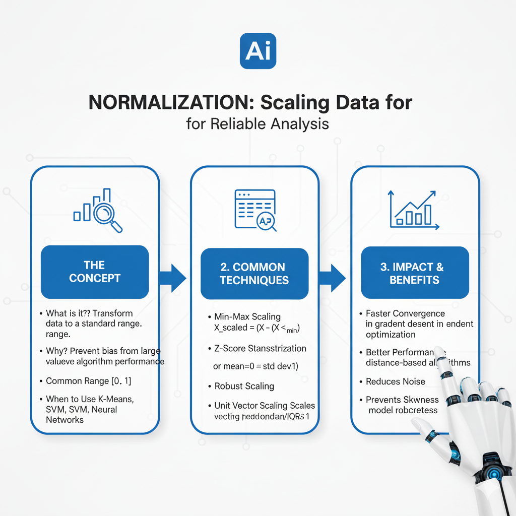
Normalization is a fundamental data preprocessing technique in machine learning and statistics. It involves rescaling the numeric features in a dataset to a standard, common range, typically between 0 and 1 or to have a mean of 0 and a standard deviation of 1. This process does not change the distribution of the data or the relationships between data points; it simply puts all features on a level playing field. By doing so, Normalization ensures that no single feature dominates the learning process simply due to its scale, leading to faster, more stable, and often more accurate machine learning models.
Part 1: Why Do We Need Normalization? The Core Reasons
The need for Normalization becomes apparent when we understand how many machine learning algorithms work under the hood. It’s not just a “good practice”; for many models, it’s a critical requirement.
1.1 Gradient-Based Algorithms and Convergence Speed
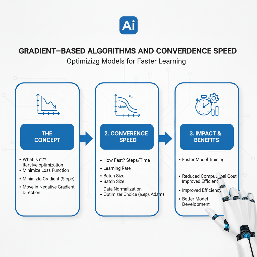
Many powerful algorithms, such as Linear Regression, Logistic Regression, and Neural Networks, use gradient descent to find the optimal model parameters. Gradient descent is an iterative process that moves step-by-step towards the minimum of a cost function (the model’s error).
- The Problem: Features with larger value ranges produce larger gradients. This forces the algorithm to take tiny, cautious steps along the axis of the high-range feature and larger, more haphazard steps along the axis of the low-range feature. The path to the minimum becomes a zig-zagging, inefficient journey, drastically slowing down convergence.
- The Solution with Normalization: When all features are on the same scale, the cost function becomes more symmetrical and “round.” The gradient descent algorithm can take uniform, confident steps in all directions, converging to the minimum much faster. This is often visualized as a smooth path down a bowl-shaped curve versus a jagged path down a narrow, elongated canyon.
1.2 Distance-Based Algorithms and Skewed Calculations
Algorithms that rely on calculating distances between data points are profoundly sensitive to feature scales.
- The Problem: Consider K-Nearest Neighbors (KNN) or K-Means Clustering. The Euclidean distance between two points is heavily dominated by the feature with the largest scale. In our house example, a difference of 2000 in square footage would completely overshadow a difference of 2 in the number of bedrooms, even though both could be equally important.
- The Solution with Normalization: After Normalization, a one-unit change in any feature is treated as equally significant. This ensures that the distance metric truly reflects the multi-dimensional similarity between data points, which is the entire basis for these algorithms.
1.3 Regularization and Fair Penalization
Algorithms that use regularization (like L1 and L2 in Linear Regression) apply a penalty to the size of the model’s coefficients to prevent overfitting.
- The Problem: If features are not normalized, a feature with a large scale (e.g., square footage) will naturally have a smaller coefficient, while a feature with a small scale (e.g., bedrooms) will have a larger coefficient, even if their true importance is similar. The regularization penalty will unfairly target the coefficient for the ‘bedrooms’ feature because it’s larger, potentially shrinking a useful predictor into irrelevance.
- The Solution with Normalization: When all features are on the same scale, the size of a coefficient becomes a direct indicator of the feature’s importance. The regularization penalty can then be applied fairly across all coefficients, correctly shrinking less important features regardless of their original scale.
Part 2: Key Normalization Techniques and When to Use Them
There is no single “best” Normalization method. The right choice depends on your data’s distribution and the algorithm you plan to use. Here are the most common techniques.
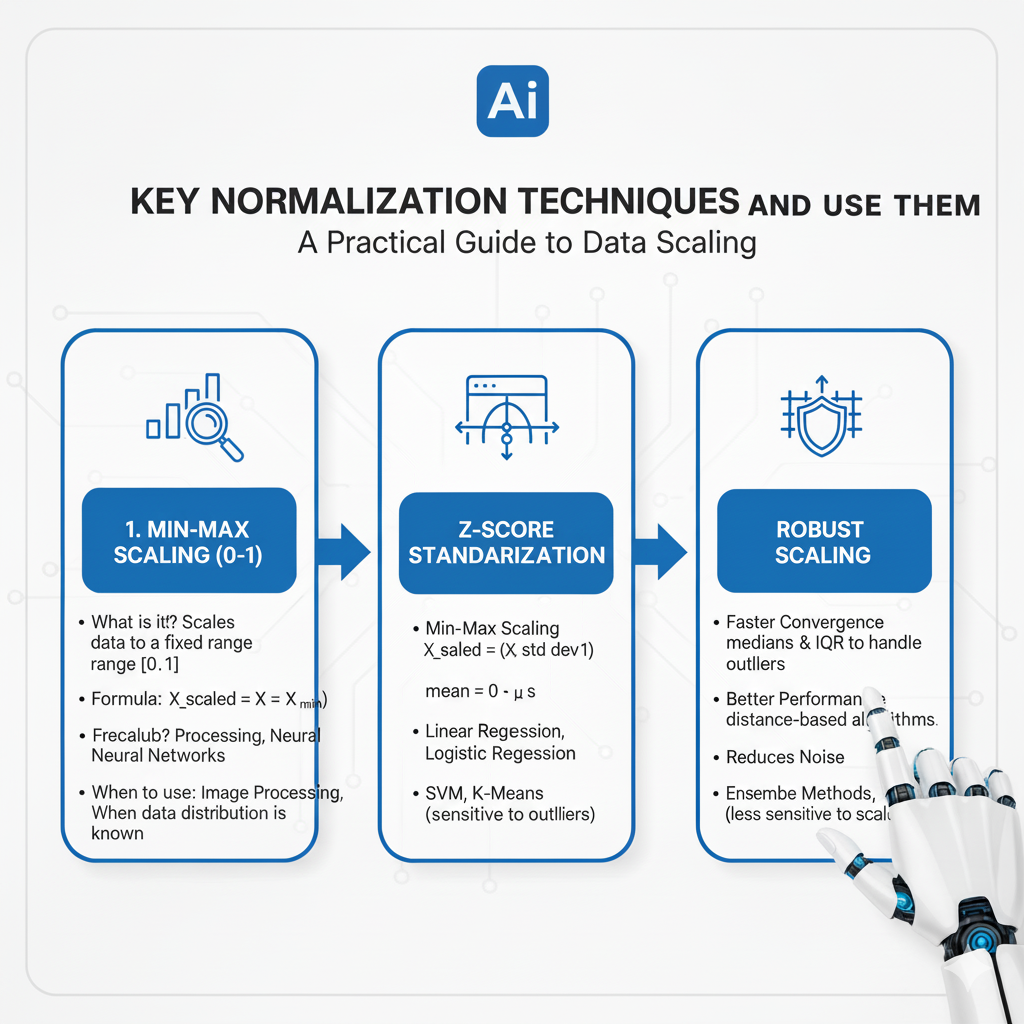
2.1 Min-Max Scaling
This is one of the simplest and most common techniques. It rescales the data to a fixed range, usually [0, 1].
- Formula: Xnorm=X−XminXmax−XminXnorm=Xmax−XminX−Xmin
- How it works: It subtracts the minimum value of the feature and then divides by the range (max-min). A value of 0 becomes the smallest observed value, and 1 becomes the largest.
- Best for: When you know the data is bounded and does not contain significant outliers. It’s commonly used in image processing (where pixel intensities are between 0-255) and neural networks when data needs to be fed into activation functions like the sigmoid, which also output in the [0,1] range.
- Drawback: It is highly sensitive to outliers. A single extreme value (an outlier) can compress the rest of the data into a very small interval.
2.2 Standardization (Z-Score Normalization)
This technique does not bound the data to a specific range. Instead, it transforms the data to have a mean of 0 and a standard deviation of 1.
- Formula: Xstd=X−μσXstd=σX−μ
where μμ is the mean and σσ is the standard deviation. - How it works: It centers the data around zero (by subtracting the mean) and scales it based on the spread of the data (by dividing by the standard deviation).
- Best for: Many machine learning algorithms, especially those that assume data is centered (like Principal Component Analysis – PCA). It is much less sensitive to outliers than Min-Max scaling because the standard deviation is influenced by outliers, but the transformation itself doesn’t force the data into a tight, fixed range.
- Drawback: The resulting data is not bounded to a fixed interval, which can be a problem for some neural network layers.
2.3 Robust Scaling
This method is designed to be robust to the presence of outliers.
- Formula: Xrobust=X−Median(X)IQR(X)Xrobust=IQR(X)X−Median(X)
where IQR is the Interquartile Range (75th percentile – 25th percentile). - How it works: It uses the median and the IQR, which are robust statistics not influenced by extreme values. The data is centered around the median and scaled by the spread of the middle 50% of the data.
- Best for: Datasets with significant outliers. If your data has many extreme values, Robust Scaling will prevent them from distorting the transformation for the rest of your data.
- Drawback: The transformed data is less interpretable than Min-Max or Z-score, as the range is not standard.
2.4 Max Abs Scaling
This scales each feature by its maximum absolute value.
- Formula: Xscaled=X∣Xmax∣Xscaled=∣Xmax∣X
- How it works: It divides each data point by the maximum absolute value found in that feature. This results in a range of [-1, 1]. It does not shift/center the data, so it preserves sparsity (zeros remain zero).
- Best for: Data that is already centered around zero or sparse data (like data from text processing using TF-IDF).
Part 3: A Practical Walkthrough: Normalizing a Sample Dataset
Let’s make this concrete with a simple example. We have a small dataset with two features: Age and Income.
Raw Data:
| Person | Age | Income ($) |
|---|---|---|
| A | 25 | 40,000 |
| B | 40 | 80,000 |
| C | 55 | 120,000 |
| D | 32 | 55,000 |
Step 1: Apply Min-Max Scaling (to [0,1])
- For
Age: Min = 25, Max = 55, Range = 30- Person A: (25-25)/30 = 0.00
- Person B: (40-25)/30 = 0.50
- Person C: (55-25)/30 = 1.00
- Person D: (32-25)/30 = 0.23
- For
Income: Min = 40,000, Max = 120,000, Range = 80,000- Person A: (40,000-40,000)/80,000 = 0.00
- Person B: (80,000-40,000)/80,000 = 0.50
- Person C: (120,000-40,000)/80,000 = 1.00
- Person D: (55,000-40,000)/80,000 = 0.19
Min-Max Scaled Data:
| Person | Age | Income |
|---|---|---|
| A | 0.00 | 0.00 |
| B | 0.50 | 0.50 |
| C | 1.00 | 1.00 |
| D | 0.23 | 0.19 |
Now, both features are on an identical 0-to-1 scale. Notice how the relative relationships are preserved.
Step 2: Apply Standardization (Z-Score)
- For
Age: Mean (μ) = 38, Standard Deviation (σ) ≈ 12.12- Person A: (25-38)/12.12 ≈ -1.07
- Person B: (40-38)/12.12 ≈ 0.17
- Person C: (55-38)/12.12 ≈ 1.40
- Person D: (32-38)/12.12 ≈ -0.50
- For
Income: Mean (μ) = 73,750, Standard Deviation (σ) ≈ 32,336- Person A: (40,000-73,750)/32,336 ≈ -1.04
- Person B: (80,000-73,750)/32,336 ≈ 0.19
- Person C: (120,000-73,750)/32,336 ≈ 1.43
- Person D: (55,000-73,750)/32,336 ≈ -0.58
Standardized Data:
| Person | Age | Income |
|---|---|---|
| A | -1.07 | -1.04 |
| B | 0.17 | 0.19 |
| C | 1.40 | 1.43 |
| D | -0.50 | -0.58 |
The data is now centered around zero. The values represent how many standard deviations a point is from the feature’s mean.
Part 4: Normalization in the Machine Learning Pipeline
Implementing Normalization correctly is as important as choosing the right technique. A critical mistake is data leakage.
4.1 The Golden Rule: Fit on Training, Transform on Training and Test Sets
You must never use information from your test set to normalize your training data. This would “leak” information about the test set into the model training process, giving you an overly optimistic and invalid performance estimate.
The correct procedure is:
- Split your data into Training and Test sets.
- Calculate the parameters for normalization (e.g., min/max, mean/std) using only the Training set.
- Apply the transformation (using the parameters from step 2) to the Training set.
- Apply the same transformation (using the same parameters from step 2) to the Test set.
You do not recalculate the min, max, or mean for the test set. It must be transformed as an unseen, new dataset would be.
4.2 Implementation in Code (Python)
Using scikit-learn makes this process safe and easy, as it enforces this good practice with its fit and transform paradigm.
python
from sklearn.model_selection import train_test_split
from sklearn.preprocessing import StandardScaler, MinMaxScaler
import pandas as pd

# Sample Data
data = {'Age': [25, 40, 55, 32], 'Income': [40000, 80000, 120000, 55000]}
df = pd.DataFrame(data)

# 1. Split the data
X_train, X_test = train_test_split(df, test_size=0.25, random_state=42)

# 2. Initialize the scaler and FIT it on the training data only
scaler = StandardScaler()
scaler.fit(X_train) # Learns the mean and std of X_train

# 3. TRANSFORM both the training and test data
X_train_scaled = scaler.transform(X_train)
X_test_scaled = scaler.transform(X_test) # Uses the mean/std from X_train

# The scaled data is a numpy array. We can convert it back to a DataFrame.
X_train_scaled = pd.DataFrame(X_train_scaled, columns=X_train.columns)
X_test_scaled = pd.DataFrame(X_test_scaled, columns=X_test.columns)

print("Original Training Data:\n", X_train)
print("\nStandardized Training Data:\n", X_train_scaled)
Part 5: When Not to Normalize
While Normalization is crucial in many scenarios, it is not always necessary.
- Tree-Based Algorithms: Algorithms like Decision Trees, Random Forests, and Gradient Boosting Machines (XGBoost, LightGBM) are based on splitting data on conditions (e.g.,
Age < 30). The scale of the features does not affect the model’s ability to find a split, so Normalization is not required. A feature with a larger range is not given any implicit preference. - When Interpretability is Key: If you need to interpret the actual values of your features in their original context (e.g., dollars, years), working with normalized data can make this more difficult.
- Data with a Native Common Scale: If all your features are already measured on the same scale and have similar distributions (e.g., all are percentages from 0-100), Normalization may offer little benefit.
Part 5: Beyond Basics – Advanced Normalization and Transformation Techniques
While Min-Max and Standardization are foundational, real-world data often demands more sophisticated techniques. These methods handle complex data distributions and specific use cases.
5.1 L1 and L2 Normalization (Vector Norm)
This technique is used per sample (row) rather than per feature (column). It scales individual data points to have a unit norm, which is essential for text data or any use case where the direction of the data vector is more important than its magnitude.
- L2 Normalization (Euclidean): Rescales a vector so that its L2 norm (Euclidean length) is 1.
- Formula: Xnorm=X∣∣X∣∣2Xnorm=∣∣X∣∣2X where ∣∣X∣∣2=∑xi2∣∣X∣∣2=∑xi2
- Use Case: Used in text classification with TF-IDF or Bag-of-Words models, and in image processing for SIFT and HOG features. It ensures that all documents or images have the same “strength” regardless of their original length or pixel intensity sum.
- L1 Normalization (Manhattan): Rescales a vector so that its L1 norm (sum of absolute values) is 1.
- Formula: Xnorm=X∣∣X∣∣1Xnorm=∣∣X∣∣1X where ∣∣X∣∣1=∑∣xi∣∣∣X∣∣1=∑∣xi∣
- Use Case: Often used to convert data into a probability distribution, as the resulting vector sums to 1. Helpful for interpreting feature importance per sample.
5.2 Power Transforms: Tackling Non-Normal Distributions
Many models assume data is roughly normally distributed. Power transforms can help reshape data to be more Gaussian-like.
- Box-Cox Transform: A parametric transformation that finds the best lambda (λ) parameter to make the data as normal as possible.
- Formula: X(λ)=Xλ−1λX(λ)=λXλ−1 for λ ≠ 0, and ln(X)ln(X) for λ = 0
- Limitation: Only works with positive data. Crucial for fixing heteroscedasticity (non-constant variance) in regression problems.
- Yeo-Johnson Transform: An extension of Box-Cox that works with both positive and negative data, making it more versatile for real-world datasets.
5.3 Quantile Transformation
This is a powerful, non-parametric method that maps the data to a specified distribution (like normal or uniform) based on quantiles.
- How it works: It sorts the data, computes quantiles, and then maps the original values to the target distribution. This can effectively handle outliers and make the data strictly follow the chosen distribution.
- Use Case: When you need your data to follow a specific distribution for statistical tests or certain models. Excellent for making non-linear data more linear.
Part 6: Industry-Specific Applications of Normalization
Different industries face unique data challenges where normalization proves essential.
6.1 Finance and Fraud Detection
- Challenge: Financial data spans multiple scales – transaction amounts ($10 to $1,000,000), account ages (days to decades), login frequencies.
- Application: Standardization is crucial for anomaly detection algorithms. Without normalization, a $1M transaction would dominate the distance calculations, making it impossible to detect subtle patterns like unusual login times or sequence of activities that indicate fraud.
6.2 Healthcare and Medical Diagnostics
- Challenge: Patient data includes lab values with different units and ranges – cholesterol (mg/dL), blood pressure (mmHg), age, weight.
- Application: Min-Max scaling is often used when feeding data into neural networks for disease prediction. This ensures that no single lab test dominates the model’s attention, allowing it to learn from all available biomarkers equally.
6.3 E-commerce and Recommendation Systems
- Challenge: User behavior data includes click counts (0-100), purchase amounts ($1-$5000), time spent on pages (seconds to hours).
- Application: L2 normalization is applied to user preference vectors before computing cosine similarity for collaborative filtering. This ensures recommendations aren’t biased toward users who simply interact more with the platform.
6.4 Natural Language Processing
- Challenge: Document length varies from short tweets to long research papers in TF-IDF vectors.
- Application: L2 normalization of document vectors ensures that similarity comparisons focus on word distribution patterns rather than document length, enabling accurate document retrieval and classification.
Part 7: The Data Science Workflow – Where Normalization Fits
Understanding where normalization fits in the broader data pipeline is crucial for effective implementation.
7.1 The Complete Preprocessing Pipeline
- Data Cleaning: Handle missing values, remove duplicates
- EDA & Feature Engineering: Create new features, identify relationships
- Feature Selection: Choose the most relevant features
- Normalization/Scaling: Apply chosen normalization technique ← HERE
- Dimensionality Reduction: Apply PCA or other techniques (if needed)
- Model Training: Train machine learning models
7.2 Critical Implementation Patterns
Pipeline Implementation in Python:
python
from sklearn.pipeline import Pipeline
from sklearn.impute import SimpleImputer
from sklearn.preprocessing import StandardScaler, OneHotEncoder
from sklearn.compose import ColumnTransformer
from sklearn.ensemble import RandomForestClassifier

# Define preprocessing for different data types
numeric_features = ['age', 'income', 'credit_score']
numeric_transformer = Pipeline(steps=[
    ('imputer', SimpleImputer(strategy='median')),
    ('scaler', StandardScaler())  # Normalization step
])

categorical_features = ['gender', 'education']
categorical_transformer = Pipeline(steps=[
    ('imputer', SimpleImputer(strategy='constant', fill_value='missing')),
    ('onehot', OneHotEncoder(handle_unknown='ignore'))
])

# Combine preprocessing steps
preprocessor = ColumnTransformer(
    transformers=[
        ('num', numeric_transformer, numeric_features),
        ('cat', categorical_transformer, categorical_features)
    ])

# Create complete pipeline with model
pipeline = Pipeline(steps=[
    ('preprocessor', preprocessor),
    ('classifier', RandomForestClassifier())
])

# Now fit and predict with the entire pipeline
pipeline.fit(X_train, y_train)
predictions = pipeline.predict(X_test)
Part 8: Common Pitfalls and How to Avoid Them
Even experienced data scientists can make critical mistakes with normalization.
8.1 Data Leakage – The Silent Killer
- Pitfall: Calculating normalization parameters (mean, std, min, max) on the entire dataset before splitting, or recalculating them on the test set.
- Consequence: Overly optimistic model performance that doesn’t generalize to real-world data.
- Solution: Always use scikit-learn’s Pipeline or ensure you only fit scalers on training data.
8.2 Normalizing Categorical Variables
- Pitfall: Applying normalization to one-hot encoded or label-encoded categorical variables.
- Consequence: Destroying the meaningful structure of categorical data and introducing false numerical relationships.
- Solution: Only normalize continuous numerical features. Use proper encoding (One-Hot, Label) for categorical variables.
8.3 Incorrect Assumptions About Data Distribution
- Pitfall: Blindly applying Standardization to heavily skewed data or data with extreme outliers.
- Consequence: The “normalized” data still has problematic distribution characteristics.
- Solution: Always visualize your data distribution first. Use Q-Q plots to check normality. Consider Robust Scaling or power transforms for skewed data.
8.4 Normalizing Binary Features
- Pitfall: Applying normalization to binary (0/1) features.
- Consequence: Unnecessarily complicating the feature space without meaningful benefit.
- Solution: Binary features typically don’t need normalization as they’re already on a comparable scale.
Part 9: Normalization in Deep Learning and Neural Networks
Normalization takes on even greater importance in deep learning, leading to specialized techniques.
9.1 Batch Normalization
A groundbreaking technique that normalizes the inputs to each layer within the network during training.
- How it works: For each mini-batch, it calculates the mean and variance of the layer’s inputs and normalizes them. It then adds two learnable parameters (scale and shift) to maintain representational power.
- Benefits:
- Allows use of higher learning rates
- Reduces sensitivity to weight initialization
- Acts as a regularizer, reducing overfitting
- Dramatically speeds up training convergence
9.2 Layer Normalization
Similar to Batch Normalization but operates across features rather than across batch examples.
- Use Case: Particularly effective for recurrent neural networks (RNNs/LSTMs) and transformer architectures where batch sizes may be small or variable.
9.3 Instance and Group Normalization
- Instance Normalization: Normalizes each channel in each sample independently. Excellent for style transfer and generative models.
- Group Normalization: Divides channels into groups and normalizes within each group. Effective when batch sizes must be small.
Part 10: Best Practices and Future Trends
10.1 Practical Guidelines for Practitioners
- Start Simple: Begin with Standardization for most cases, Min-Max for bounded data/neural networks.
- Visualize Always: Plot distributions before and after normalization to understand the transformation.
- Algorithm-Specific Choices:
- Gradient-Based Methods: Always normalize (Standardization typically best)
- Distance-Based Methods: Always normalize (Standardization or Min-Max)
- Tree-Based Methods: Usually not needed
- Neural Networks: Always normalize + consider Batch Normalization
- Monitor Impact: Compare model performance with and without normalization to validate its necessity.
10.2 Emerging Trends and Future Directions
- Automated Normalization: ML platforms that automatically test multiple normalization strategies and select the optimal one for a given dataset and model.
- Adaptive Normalization: Techniques that learn the optimal normalization strategy during model training rather than being fixed in preprocessing.
- Domain-Specific Normalization: Specialized normalization methods emerging for particular data types like graph data, 3D point clouds, and time series with irregular sampling.
- Federated Learning Normalization: Techniques for normalizing data across distributed devices without centralizing the data, preserving privacy while maintaining model performance.
Conclusion: A Simple Step for Model Excellence
Normalization is a deceptively simple yet profoundly impactful step in the data preprocessing pipeline. It is the process of translating diverse data languages into a common tongue that our machine learning models can understand without bias. By ensuring that all features contribute equally to the learning process, it paves the way for faster training, more stable models, and more reliable results.
Mastering when and how to apply techniques like Min-Max Scaling, Standardization, and Robust Scaling is a hallmark of a skilled data practitioner. It transforms the raw, chaotic numbers of a dataset into a refined, harmonious input, ultimately simplifying your data to build far better models.