What Is ANOVA? Simplified Explanation with Real-World Examples

What is ANOVA? Learn how Analysis of Variance works with simple explanations & real-world examples. Understand types, F-tests, assumptions, and interpretation. Master ANOVA today

Introduction: Beyond the T-Test – The Need for Comparing Multiple Groups

In both scientific research and business analytics, a fundamental question often arises: Are there differences between the means (averages) of several groups? Imagine a pharmaceutical company testing three new dosages of a drug. An agricultural scientist comparing crop yields for four different fertilizers. A marketing manager evaluating the effectiveness of five different advertising campaigns.

The intuitive approach might be to perform multiple t-tests, comparing each group to every other group (Drug A vs. B, A vs. C, B vs. C). However, this method has a critical flaw: the problem of inflated Type I errors. Simply put, the more comparisons you make, the higher the chance you’ll stumble upon a “statistically significant” difference purely by accident, like finding a pattern in random noise.

This is where ANOVA comes to the rescue. ANOVA, which stands for Analysis of Variance, is a powerful statistical technique developed by Ronald Fisher in the early 20th century. It allows you to compare the means of three or more groups simultaneously to determine if at least one of them is statistically significantly different from the others. It does this by analyzing the variances within the data, hence its name.

This article will demystify ANOVA. We will break down its core logic, explore its different types, walk through a real-world calculation, and interpret its results, all with the goal of making this essential statistical tool accessible and practical.

Part 1: The Core Logic of ANOVA – Untangling Two Types of Variance

At its heart, ANOVA answers a simple question: Is the variation between the different group means large compared to the variation within the individual groups?

To understand this, let’s visualize two scenarios for our drug efficacy example, where we measure a health outcome (a higher score is better).

Scenario A: The Drugs Are Truly Different

• Drug A Group: Scores are all clustered tightly around 70.
• Drug B Group: Scores are all clustered tightly around 80.
• Drug C Group: Scores are all clustered tightly around 90.

Here, the variation between the groups is large (the group averages of 70, 80, and 90 are spread out). The variation within each group is small (the scores in each group are very consistent). In this case, ANOVA would likely tell us that there is a statistically significant difference between the drugs.

Scenario B: The Drugs Are Not Different

• Drug A Group: Scores are scattered from 50 to 90.
• Drug B Group: Scores are scattered from 55 to 85.
• Drug C Group: Scores are scattered from 60 to 95.

Here, the variation between the groups is small (the group averages might all be around 75). The variation within each group is huge. The scores are so wildly variable within each group that the differences between the group averages look trivial and could easily be due to random chance. ANOVA would likely tell us there is no significant difference.

ANOVA formalizes this intuition by calculating two key quantities:

1. Mean Square Between (MSB): This measures the variance between the groups. It quantifies how much the group means deviate from the overall grand mean (the average of all data points). A large MSB suggests the groups are being pulled apart by some factor.
2. Mean Square Within (MSW or MSE): This measures the variance within the groups. It’s essentially an average of the variances within each group. It represents the inherent “noise” or random error in the data. A large MSW makes it harder to detect a true signal.

Part 2: The ANOVA F-Test – The Heart of the Matter

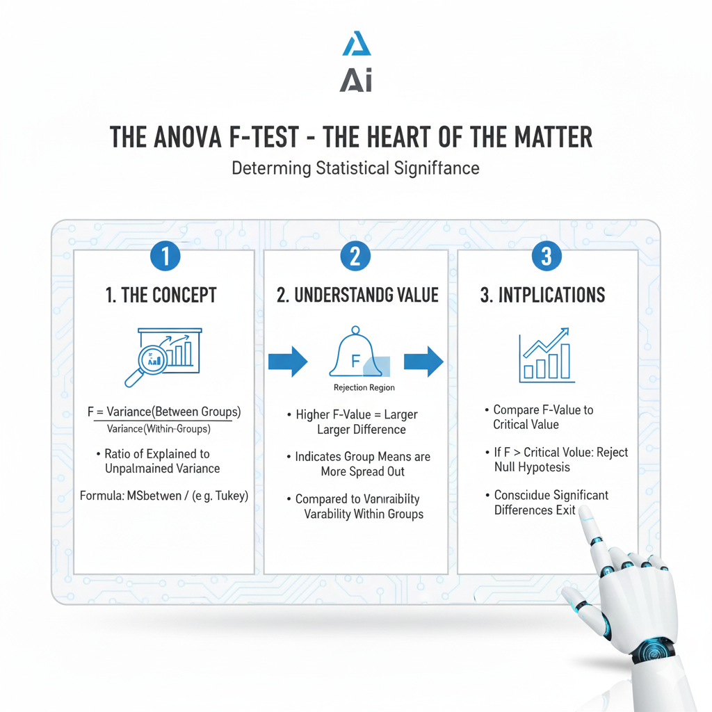
ANOVA uses these two variance estimates to calculate a single test statistic: the F-statistic.

F = Mean Square Between (MSB) / Mean Square Within (MSW)

The F-statistic is a ratio. It asks: “How many times larger is the variance between the groups than the variance within the groups?”

• F is close to 1: If the F-statistic is around 1, it means the variance between groups is roughly equal to the variance within groups. This suggests that the group means are not significantly different. The observed differences are likely just random noise.
• F is significantly greater than 1: If the F-statistic is much larger than 1, it means the variance between groups is much larger than the variance within groups. This provides evidence that at least one group mean is statistically significantly different from the others. The factor you’re testing (e.g., drug type, fertilizer brand) is having a real effect.

But how do we know what “significantly greater than 1” means? This is where the p-value comes in. The F-statistic follows a specific distribution known as the F-distribution. Statistical software (or F-tables) uses the calculated F-value and the degrees of freedom associated with MSB and MSW to find a p-value.

• If p-value < significance level (e.g., 0.05): We reject the null hypothesis. We conclude that there is a statistically significant difference between at least two of the group means.
• If p-value > significance level (e.g., 0.05): We fail to reject the null hypothesis. We do not have enough evidence to say that the group means are different.

Crucially, a significant ANOVA result does NOT tell you which specific groups are different. It only tells you that at least one difference exists. To find out where those differences lie, you need to conduct post-hoc tests.

Part 3: The Different Flavors of ANOVA

ANOVA is a family of techniques. The type you use depends on the structure of your experiment and the number of factors you are investigating.

3.1 One-Way ANOVA

This is the simplest and most common form. It is used when you are comparing the means of three or more groups based on one single independent variable (also called a “factor”).

• Independent Variable (Factor): Drug Dosage
• Levels/Groups: Level 1 (Placebo), Level 2 (50mg), Level 3 (100mg), Level 4 (150mg)
• Dependent Variable: Patient Recovery Score (a continuous measure).

A One-Way ANOVA would tell you if dosage level has a significant effect on recovery scores.

3.2 Two-Way ANOVA

This is used when you want to analyze the effect of two independent variables simultaneously. It’s far more powerful because it can also test for interactions between the factors.

• Independent Variable 1: Drug Dosage (Placebo, 50mg, 100mg)
• Independent Variable 2: Patient Age Group (Young, Middle-aged, Senior)
• Dependent Variable: Patient Recovery Score.

A Two-Way ANOVA can answer three questions:

1. Main Effect of Dosage: Is there a significant difference in recovery scores between the dosage levels, ignoring age?
2. Main Effect of Age Group: Is there a significant difference in recovery scores between the age groups, ignoring dosage?
3. Interaction Effect between Dosage and Age: Does the effect of the drug dosage depend on the patient’s age? For example, maybe the 100mg dosage works great for young patients but is ineffective for seniors. This interaction effect is often the most insightful finding.

3.3 Other Types

• Repeated Measures ANOVA: Used when the same subjects are measured multiple times under different conditions (e.g., measuring patient blood pressure before, during, and after treatment).
• MANOVA (Multivariate ANOVA): Used when you have multiple dependent variables (e.g., you want to test the effect of a fertilizer on both plant height and leaf area simultaneously).

Part 4: A Real-World Walkthrough – The Marketing Campaign Example

Let’s solidify our understanding with a detailed, hypothetical example.

Scenario: A company runs three different marketing campaigns (Campaign A, B, and C) to boost weekly sales. They randomly assign the campaigns to different, comparable regions and collect the sales data (in thousands of dollars).

The Data:

• Campaign A: [22, 26, 24, 28, 25] | Mean = 25
• Campaign B: [30, 29, 31, 32, 28] | Mean = 30
• Campaign C: [25, 23, 27, 24, 26] | Mean = 25

The Grand Mean (average of all 15 data points) = 26.67

Step 1: State the Hypotheses

• Null Hypothesis (H₀): μ_A = μ_B = μ_C (The mean sales for all three campaigns are equal).
• Alternative Hypothesis (H₁): At least one campaign mean is different.

Step 2: Calculate the Variances (The “Analysis of Variance”)

We will calculate the Sum of Squares (SS), degrees of freedom (df), and Mean Squares (MS). While software does this instantly, walking through the concepts is invaluable.

1. Sum of Squares Between (SSB): How much the group means deviate from the grand mean.
   • For each group, calculate: (Group Mean – Grand Mean)², then multiply by the number of observations in that group.
   • SSB = 5*(25-26.67)² + 5*(30-26.67)² + 5*(25-26.67)² = 83.33
2. Sum of Squares Within (SSW): How much the individual data points deviate from their own group mean.
   • For each data point, calculate: (Data Point – Its Group Mean)², then sum them all.
   • SSW = (22-25)² + (26-25)² + … + (24-25)² + (26-25)² = 54
3. Total Sum of Squares (SST): SSB + SSW = 83.33 + 54 = 137.33
4. Degrees of Freedom (df):
   • df-between: Number of groups – 1 = 3 – 1 = 2
   • df-within: Total number of observations – Number of groups = 15 – 3 = 12
   • df-total: 15 – 1 = 14
5. Mean Squares (MS): The average variance.
   • MSB = SSB / df-between = 83.33 / 2 = 41.67
   • MSW = SSW / df-within = 54 / 12 = 4.5

Step 3: Compute the F-Statistic

F = MSB / MSW = 41.67 / 4.5 = 9.26

Step 4: Make a Decision

We compare our calculated F-value of 9.26 to a critical F-value from a statistical table for F(2, 12) degrees of freedom at a 0.05 significance level. The critical value is approximately 3.89.

• Since 9.26 > 3.89, we reject the null hypothesis.

Furthermore, statistical software would give us a p-value for F=9.26 with df(2,12). This p-value would be approximately 0.004.

• Since p-value (0.004) < 0.05, we reject the null hypothesis.

Conclusion: There is a statistically significant difference in mean weekly sales between at least two of the three marketing campaigns.

Part 5: After a Significant ANOVA – The Crucial Next Step

Our ANOVA told us that not all campaigns are equal, but it didn’t tell us which ones are different. Is B better than A and C? Are A and C the same? To answer this, we perform post-hoc tests. These are specialized tests designed to make multiple comparisons between groups while controlling for the Type I error inflation we mentioned at the beginning.

Common post-hoc tests include Tukey’s HSD (Honestly Significant Difference), Bonferroni correction, and Scheffé’s method.

If we run a Tukey’s HSD test on our data, it might produce an output like this:

Comparison	Mean Difference	p-value	Significant?
Campaign B – Campaign A	5.0	0.005	Yes
Campaign B – Campaign C	5.0	0.005	Yes
Campaign C – Campaign A	0.0	0.999	No

Final Interpretation: The ANOVA (F(2,12)=9.26, p=0.004) indicated a significant overall difference. Post-hoc Tukey HSD tests revealed that Campaign B led to significantly higher sales than both Campaign A and Campaign C (p<0.05 for both), which were not significantly different from each other. The marketing team should allocate the budget to Campaign B.

Part 6: Key Assumptions of ANOVA

For the results of an ANOVA to be valid, the data must meet certain assumptions:

1. Independence of Observations: The data points in different groups must be independent. This is usually achieved through random sampling or random assignment to groups.
2. Normality: The data within each group should be approximately normally distributed. ANOVA is somewhat robust to minor violations of this assumption, especially with larger sample sizes.
3. Homogeneity of Variances (Homoscedasticity): The variance within each of the groups should be roughly equal. This can be tested using Levene’s Test or Bartlett’s Test.

If these assumptions are violated, non-parametric alternatives like the Kruskal-Wallis test (the non-parametric version of One-Way ANOVA) can be used.

Part 7: ANOVA in Action – Advanced Real-World Applications Across Industries

The utility of ANOVA extends far beyond basic scientific experiments. Let’s explore how different industries leverage this powerful technique to solve complex problems and drive decision-making.

7.1 Manufacturing and Quality Control

Scenario: An automotive parts manufacturer wants to determine if there is a difference in the tensile strength of metal rods produced on four different production lines.

• Factor: Production Line (Line 1, Line 2, Line 3, Line 4)
• Dependent Variable: Tensile Strength (measured in MPa)
• Application: A One-Way ANOVA can identify if any specific production line is producing weaker or stronger rods. If a significant difference is found, a post-hoc test pinpoints which lines differ. This allows the quality team to focus their investigation on specific machinery, operators, or raw material batches, saving time and resources while improving overall product consistency.

7.2 Education and Psychology

Scenario: A educational researcher is studying the effectiveness of three different teaching methods (Traditional Lecture, Flipped Classroom, Project-Based Learning) on student final exam scores. They suspect that the effectiveness might also depend on the students’ primary learning style (Visual, Auditory, Kinesthetic).

• Factor 1: Teaching Method
• Factor 2: Learning Style
• Dependent Variable: Final Exam Score
• Application: This calls for a Two-Way ANOVA. It can answer:
  1. Is there a main effect of Teaching Method? (Does one method lead to higher scores overall?)
  2. Is there a main effect of Learning Style? (Do visual learners outperform others overall?)
  3. Is there an interaction effect? (For example, perhaps kinesthetic learners perform dramatically better in the Project-Based Learning group, but worse in the Traditional Lecture group). This interaction is often the most valuable insight, enabling personalized educational strategies.

7.3 Business and Marketing

Scenario: An e-commerce company tests a new website layout. They want to understand how the layout affects user behavior, measured by two key metrics: “Time Spent on Site” and “Purchase Conversion Rate.”

• Factors: Website Layout (Old vs. New), Customer Segment (New vs. Returning)
• Dependent Variables: Time Spent on Site, Purchase Conversion Rate
• Application: A MANOVA (Multivariate Analysis of Variance) is used here. Unlike standard ANOVA, MANOVA can handle multiple related dependent variables simultaneously. This is crucial because user behaviors are often correlated. MANOVA can determine if the new website layout has a statistically significant overall effect on the combination of user engagement and conversion, preventing the inflated error rate that would come from running two separate ANOVAs.

Part 8: A Practical Guide to Running ANOVA – From Software to Interpretation

Understanding the theory is one thing; executing it correctly is another. Here is a step-by-step guide to performing an ANOVA in practice, using statistical software like R, Python, or SPSS.

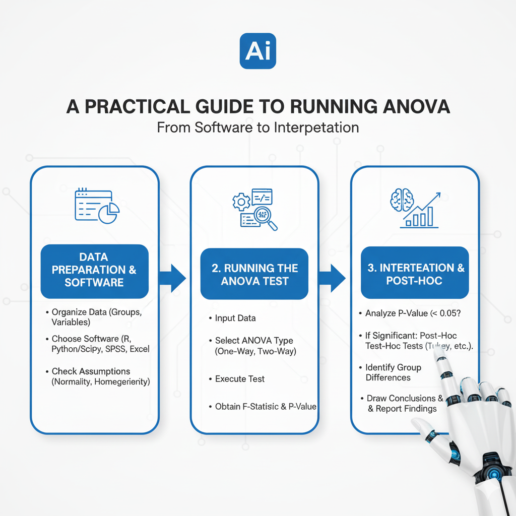
8.1 The Pre-Analysis Checklist

Before you even run the test, complete this checklist:

1. Data Structure: Ensure your data is in the correct format—typically one column for the grouping (factor) variable and one for the continuous dependent variable.
2. Assumption Checking:
   • Normality: Create Q-Q plots or run Shapiro-Wilk tests for each group.
   • Homogeneity of Variances: Run Levene’s Test. A non-significant p-value (p > 0.05) suggests the assumption is met.
   • Independence: This is determined by your experimental design (e.g., random assignment).

8.2 Sample Code and Output Interpretation

In R:

r

# One-Way ANOVA
my_data <- read.csv("marketing_data.csv")
model <- aov(sales ~ campaign, data = my_data)
summary(model)

# Check assumptions
plot(model, 1) # Checks homoscedasticity
library(car)
leveneTest(sales ~ campaign, data = my_data)

# If ANOVA is significant, run Tukey HSD
TukeyHSD(model)

In Python (using scipy and statsmodels):

python

import scipy.stats as stats
import pandas as pd
import statsmodels.api as sm
from statsmodels.formula.api import ols
from statsmodels.stats.multicomp import pairwise_tukeyhsd

# One-Way ANOVA
df = pd.read_csv('marketing_data.csv')
f_stat, p_value = stats.f_oneway(df[df['campaign']=='A']['sales'],
                                 df[df['campaign']=='B']['sales'],
                                 df[df['campaign']=='C']['sales'])
print(f"F-statistic: {f_stat:.2f}, p-value: {p_value:.4f}")

# Using statsmodels for a more detailed table
model = ols('sales ~ C(campaign)', data=df).fit()
anova_table = sm.stats.anova_lm(model, typ=2)
print(anova_table)

# Tukey HSD
tukey = pairwise_tukeyhsd(endog=df['sales'], groups=df['campaign'], alpha=0.05)
print(tukey)

Interpreting the Output:
A typical ANOVA table looks like this:

Source	Sum Sq	df	Mean Sq	F value	p-value
Campaign	83.33	2	41.67	9.26	0.004**
Residuals	54.00	12	4.50

You would report this as: “A one-way ANOVA was conducted to compare the effect of marketing campaign on sales. There was a statistically significant difference in sales between at least two campaigns (F(2, 12) = 9.26, p = .004).”

Part 9: Common Pitfalls and How to Avoid Them

Even experienced analysts can make mistakes when using ANOVA. Here are the most common pitfalls and how to steer clear of them.

1. Ignoring Violated Assumptions:
   • Pitfall: Running ANOVA on data that is clearly non-normal or has unequal variances.
   • Consequence: Increased risk of Type I or Type II errors (false positives or false negatives).
   • Solution: Always test assumptions first. If variances are unequal, use a Welch’s ANOVA correction (available in most software). If normality is severely violated, use the non-parametric Kruskal-Wallis test.
2. Treating a Significant ANOVA as a Final Answer:
   • Pitfall: Concluding “all groups are different” after a significant omnibus ANOVA.
   • Consequence: Drawing incorrect and overly broad conclusions.
   • Solution: Remember that a significant ANOVA only tells you that not all means are equal. You must perform post-hoc tests to identify which specific pairs are different.
3. The Multiple Comparisons Problem (Revisited):
   • Pitfall: After a significant ANOVA, performing multiple independent t-tests without adjustment for the post-hoc comparisons.
   • Consequence: Inflates the family-wise error rate, undermining the purpose of using ANOVA in the first place.
   • Solution: Always use a dedicated post-hoc test like Tukey’s HSD, which is specifically designed to control the overall error rate.
4. Fishing for Significance:
   • Pitfall: Measuring many different dependent variables and running an ANOVA on all of them without a prior hypothesis.
   • Consequence: High probability of finding a “significant” result by chance alone.
   • Solution: Pre-register your hypotheses and primary outcome variables before collecting data. Use MANOVA for truly related multiple outcomes.

Part 10: The Future of ANOVA and Its Place in the Modern Data Toolkit

In the age of machine learning and big data, where does a century-old technique like ANOVA stand? Its role is more relevant than ever, but it is evolving.

1. Integration with Machine Learning Pipelines:
   • ANOVA is not just for hypothesis testing; it’s a powerful feature selection tool. In datasets with hundreds of features, a One-Way ANOVA F-test can be used to rank the importance of categorical features in predicting a continuous target. This provides a fast, model-agnostic way to reduce dimensionality before feeding data into more complex algorithms like Random Forests or Gradient Boosting machines.
2. Robust and Bayesian ANOVA:
   • **Traditional ANOVA is being supplemented by more robust versions that are less sensitive to outliers and violated assumptions. Furthermore, Bayesian ANOVA is gaining traction. Instead of providing a p-value, Bayesian ANOVA provides a probability for each model (e.g., the probability that a model with a group effect is better than one without). This offers a more intuitive and direct interpretation of the evidence.
3. A Foundational Pillar, Not a Relic:
   • While techniques like mixed-effects models can handle more complex data structures (e.g., nested or hierarchical data), the core logic of ANOVA—partitioning variance—remains fundamental. Understanding ANOVA provides the conceptual groundwork for grasping these advanced models. It teaches the critical skill of thinking about the sources of variation in data, which is invaluable whether you are running a simple experiment or building a sophisticated AI.

Conclusion: ANOVA as an Indispensable Tool for Discovery

ANOVA is far more than a statistical procedure; it is a fundamental framework for comparative analysis. By elegantly separating signal (variance between groups) from noise (variance within groups), it provides a rigorous and reliable method to test hypotheses across multiple groups.

From optimizing business processes and validating scientific experiments to guiding public policy decisions, ANOVA empowers us to move from vague questions like “Do these things differ?” to confident, data-driven conclusions. Mastering its logic—understanding the F-ratio, interpreting p-values, and knowing when to apply post-hoc tests—unlocks the ability to make sense of complex, multi-faceted data, turning raw numbers into actionable intelligence.