Master clustering techniques from K-Means to DBSCAN. Learn how to group data effectively, choose the right algorithm, and apply clustering to real-world problems like customer segmentation and anomaly detection
Introduction: The Human Instinct to Group and Categorize
From a young age, we learn by grouping: we separate toys from food, animals from people, and friends from strangers. This innate desire to find order in chaos is not just a human trait; it is the very foundation of a powerful family of machine learning techniques known as Clustering.
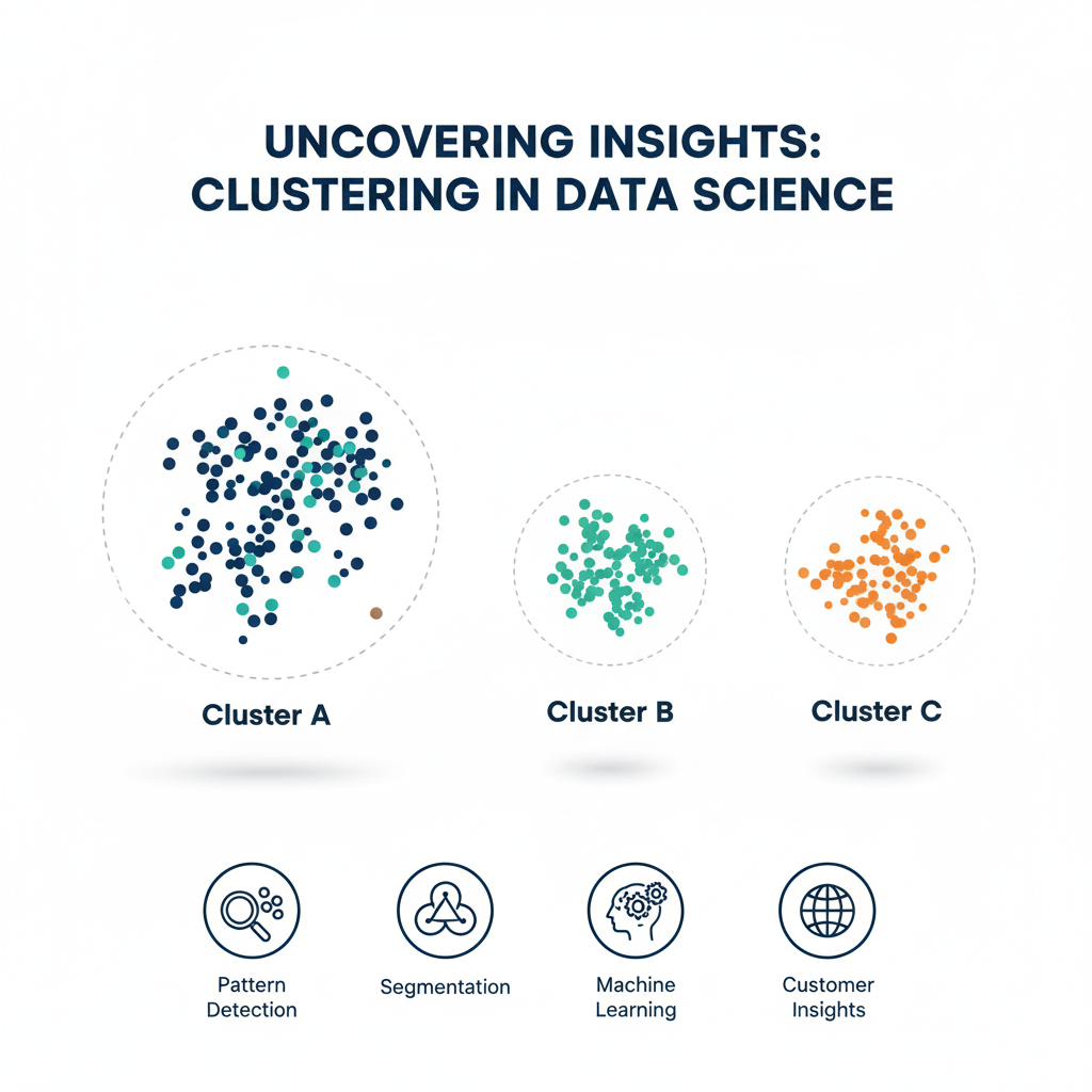
In the digital realm, Clustering is an unsupervised learning method used to partition a set of data points into groups, or “clusters,” such that points in the same cluster are more similar to each other than to those in other clusters. The goal is to discover the inherent, hidden structure within unlabeled data. Unlike supervised learning, where we have a target variable to predict, Clustering allows the data to speak for itself, revealing natural groupings and patterns that might not be immediately obvious.
Why is this important? Clustering powers a significant part of our modern digital experience. It is the engine behind:
- Customer Segmentation: Grouping customers based on purchasing behavior for targeted marketing.
- Document Categorization: Organizing news articles or scientific papers into topics.
- Anomaly Detection: Identifying fraudulent credit card transactions or network intrusions by finding data points that don’t belong to any cluster.
- Image Segmentation: Grouping pixels in an image to identify objects.
This article will demystify the world of Clustering. We will start with the fundamental concepts, then dive deep into two of the most popular and representative algorithms: the classic, centroid-based K-Means and the sophisticated, density-based DBSCAN. By comparing their strengths and weaknesses, you will gain the knowledge to choose the right tool for your data.
Part 1: The Foundation – Core Concepts of Clustering
Before exploring specific algorithms, it’s crucial to understand the universal concepts that underpin all Clustering methods.
1.1 The “Similarity” Principle
At its heart, every clustering algorithm needs a way to measure “similarity.” The most common measure is distance. Points that are close together in the feature space are considered similar and are candidates for the same cluster. The most frequently used distance metric is Euclidean Distance (the straight-line distance between two points). Other metrics include Manhattan and Cosine distance, each with its own use case.
1.2 What Defines a “Good” Cluster?
There are two primary ways to think about cluster quality:
- High Intra-cluster Similarity: Points within the same cluster should be as similar as possible (tightly packed).
- Low Inter-cluster Similarity: Points from different clusters should be as dissimilar as possible (well-separated).
The balance between these two goals is the eternal challenge of Clustering.
1.3 The Types of Clustering Algorithms
The field is vast, but algorithms can be broadly categorized:
- Centroid-based: Clusters are represented by a central vector (the centroid), which may not necessarily be an actual data point. The goal is to minimize the distance between points and their cluster centroid. K-Means is the quintessential example.
- Density-based: Clusters are defined as dense regions of data points separated by sparse regions. This is excellent for discovering clusters of arbitrary shape and handling outliers. DBSCAN is the champion of this category.
- Hierarchical-based: Creates a tree of clusters (a dendrogram), allowing users to see clusters at different levels of granularity, from a single cluster containing all points to each point being its own cluster.
- Distribution-based: Assumes data points belong to a probability distribution (like a Gaussian), and clusters are formed by grouping points that are most likely to belong to the same distribution.
Part 2: K-Means Clustering – The Centroid-Based Workhorse
K-Means is arguably the most well-known clustering algorithm due to its simplicity, efficiency, and intuitive nature.
2.1 The Intuition Behind K-Means
Imagine you have a set of points on a 2D plane. Your goal is to group them into K clusters. How would you do it? You might start by randomly placing K “centers” on the plane. Then, you would assign each data point to its nearest center. Next, you would move each center to the actual middle (mean) of the points assigned to it. You would repeat the assignment and movement steps until the centers stop moving significantly. This intuitive process is exactly the K-Means algorithm.
2.2 The Step-by-Step Algorithm
- Initialization: Choose the number of clusters, K. Randomly select K data points from the dataset as the initial centroids.
- Assignment Step: For each data point in the dataset, calculate its distance to all K centroids. Assign the point to the cluster of the nearest centroid.
- Update Step: For each cluster, recalculate its centroid as the mean (average) of all data points currently assigned to that cluster.
- Iteration: Repeat Steps 2 and 3 until one of the following is true:
- The centroids no longer change significantly.
- The assignments of points to clusters remain the same.
- A predetermined maximum number of iterations is reached.
2.3 A Concrete Example: Customer Segmentation
Let’s cluster a simple set of customers based on their Annual Income and Spending Score.
Raw Data:
| Customer | Annual Income ($000) | Spending Score (1-100) |
|---|---|---|
| A | 15 | 15 |
| B | 15 | 80 |
| C | 55 | 50 |
| D | 65 | 20 |
| E | 85 | 90 |
Let’s choose K=2 and initialize with Customers A and B as centroids.
- Iteration 1, Assignment:
- Distances to Centroid A(15,15): A:0, B:65, C:57, D:71, E:106
- Distances to Centroid B(15,80): A:65, B:0, C:50, D:78, E:71
- Cluster 1 (near A): A, C, D
- Cluster 2 (near B): B, E
- Iteration 1, Update:
- New Centroid for Cluster 1: Mean of A(15,15), C(55,50), D(65,20) = (45, 28)
- New Centroid for Cluster 2: Mean of B(15,80), E(85,90) = (50, 85)
- Iteration 2, Assignment (using new centroids):
- Cluster 1 (near (45,28)): A, D
- Cluster 2 (near (50,85)): B, C, E
- Iteration 2, Update:
- New Centroid for Cluster 1: (40, 18)
- New Centroid for Cluster 2: (52, 73)
The algorithm would continue until the centroids stabilize, revealing one cluster of low-income, low-spending customers and another with a mix of high-spending customers.
2.4 Strengths and Weaknesses of K-Means
Strengths:
- Simple and Fast: Computationally efficient, even for large datasets.
- Intuitive and Easy to Implement: The concept is easy to understand.
- Guarantees Convergence: It will always find a solution.
Weaknesses (The “K-Means Assumptions”):
- You must choose K: The most significant drawback. The algorithm doesn’t determine the number of clusters for you. Choosing the wrong K leads to poor results.
- Sensitive to Initialization: Poor initial random centroids can lead to suboptimal clustering. This is often mitigated by the “K-Means++” initialization technique.
- Assumes Spherical, Equally-Sized Clusters: It struggles with clusters of non-spherical shapes or widely different sizes, as it relies on distance to a central point.
- Sensitive to Outliers: Since centroids are calculated as means, outliers can dramatically pull the centroid away from the true cluster center.
Part 3: DBSCAN – The Density-Based Discovery Engine

While K-Means is powerful, its weaknesses make it unsuitable for many real-world datasets. This is where DBSCAN (Density-Based Spatial Clustering of Applications with Noise) shines. It abandons the concept of centroids in favor of a more natural idea: clusters are dense regions separated by empty regions.
3.1 The Core Intuition of Density
Imagine a map of a country at night. Cities appear as bright, dense clusters of light. Towns are smaller, less dense clusters. Rural areas are sparsely lit, and there are completely dark areas. DBSCAN views data in exactly this way. It doesn’t try to force every point into a cluster; it acknowledges that some points are just “noise.”
3.2 The Key Terminology and Algorithm
DBSCAN requires two parameters:
- eps (ε): The maximum distance between two points for them to be considered neighbors.
- min_samples (minPts): The minimum number of points required to form a dense region (a core point).
It classifies points into three categories:
- Core Point: A point that has at least
min_samplespoints within itsepsradius. - Border Point: A point that has fewer than
min_sampleswithin itsepsradius, but is within theepsradius of a core point. - Noise Point (Outlier): A point that is neither a core point nor a border point.
The algorithm works as follows:
- For each point in the dataset, determine if it’s a core point by counting its neighbors within
eps. - Randomly select a core point that has not been visited and form a new cluster.
- Recursively find all points that are density-reachable from this core point (i.e., all points that can be reached through a chain of core points) and add them to the cluster.
- Repeat steps 2 and 3 until all core points have been visited and assigned to clusters.
- Assign all non-core, non-border points as noise.
3.3 A Concrete Example: Spatial Points on a Map
Imagine points representing restaurant locations in a city. We want to find dense “food districts.”
- We set
epsto 500 meters andmin_samplesto 5. - A restaurant in a downtown area with 10 other restaurants within 500 meters is a Core Point.
- A restaurant on the edge of this district with only 3 neighbors within 500m, but which is within 500m of a core point, is a Border Point and is added to the downtown cluster.
- A standalone restaurant in a residential area with only 1 neighbor within 500m is classified as Noise.
DBSCAN would successfully identify the downtown food district, a separate food court at the mall, and correctly label the isolated restaurant as not belonging to any cluster.
3.4 Strengths and Weaknesses of DBSCAN
Strengths:
- Does Not Require Pre-Specifying K: It automatically discovers the number of clusters.
- Finds Clusters of Arbitrary Shape: It is not biased towards spherical clusters like K-Means.
- Robust to Outliers: It has a built-in mechanism to identify and handle noise/outliers.
- Works Well with Spatial Data: Its principles are naturally suited for geography.
Weaknesses:
- Struggles with Varying Densities: If one cluster is very dense and another is sparse, it can be difficult to find a single
epsandmin_samplesthat works for both. - Sensitive to Parameter Tuning: The choice of
epsandmin_samplesis critical and can be non-trivial. - Performance on High-Dimensional Data: The “curse of dimensionality” can make the concept of distance/density less meaningful.
Part 4: K-Means vs. DBSCAN – A Head-to-Head Comparison
Choosing between K-Means and DBSCAN is not about which is “better,” but which is more appropriate for your specific data and goal.
| Feature | K-Means | DBSCAN |
|---|---|---|
| Cluster Shape | Prefers spherical, convex shapes. | Can find arbitrarily shaped clusters. |
| Number of Clusters (K) | Must be specified by the user. | Determined automatically by the algorithm. |
| Outlier Handling | Highly sensitive; outliers pull centroids. | Robust; has an explicit noise category. |
| Data Distribution | Works best on clusters of similar size and density. | Struggles with clusters of widely varying densities. |
| Performance | Generally very fast and scalable. | Can be slower on large datasets, but efficient with spatial indexes. |
| Use Case | Customer segments, image color quantization, document grouping by topic. | Anomaly detection, spatial data analysis, finding irregular patterns. |
When to Use Which:
- Use K-Means when you have a good reason to believe the clusters are spherical, the data is relatively clean, and you have an idea of how many clusters you want (or can use methods like the Elbow Method to find K).
- Use DBSCAN when you don’t know the number of clusters, the clusters are likely to be non-spherical, you need to detect outliers, or you are working with spatial data.
Part 5: The Clustering Workflow and Best Practices
Successfully applying clustering involves more than just running an algorithm. It’s a process.

- Preprocessing is Key:
- Normalize/Standardize Your Data: Features on different scales (e.g., income in dollars and age in years) will distort distance calculations. Normalization (e.g., Min-Max Scaling) or Standardization (Z-score) is essential.
- Handle Missing Values and Outliers: Decide how to treat them based on your chosen algorithm.
- Feature Selection and Engineering: The clusters you find are entirely defined by the features you use. Choose features that are relevant to the grouping you want to discover.
- Algorithm Selection and Tuning: Based on your data’s characteristics (see the comparison above), choose an algorithm and tune its parameters. For K-Means, use the Elbow Method (plotting the within-cluster sum of squares against K) to find a good value for K. For DBSCAN, use domain knowledge and visualization (like a k-distance graph) to choose
eps. - Interpretation and Validation: This is the most challenging part. Since there is no ground truth, validation is often qualitative.
- Use Domain Knowledge: Do the clusters make sense to a business expert?
- Visualize: Plot the clusters in 2D or 3D if possible.
- Use Internal Metrics: Metrics like the Silhouette Score can quantify how well-separated the clusters are.
Part 6: Advanced Clustering Techniques and Hybrid Approaches
While K-Means and DBSCAN represent foundational approaches, modern data challenges often require more sophisticated clustering techniques. These advanced methods address specific limitations and handle complex data structures that common algorithms struggle with.
6.1 Hierarchical Clustering: The Tree of Relationships
Hierarchical clustering creates a tree-like structure of clusters, offering a multi-level perspective of data relationships that single-level algorithms cannot provide.
Two Main Approaches:
- Agglomerative (Bottom-Up): Starts with each data point as its own cluster and progressively merges the most similar clusters until only one remains. This is the most common hierarchical approach.
- Divisive (Top-Down): Begins with all points in one cluster and recursively splits them into smaller clusters.
Key Advantages:
- No Pre-specified K Required: The dendrogram visualization allows users to choose an appropriate clustering level after seeing the full hierarchy.
- Rich Visual Representation: Dendrograms provide intuitive insights into data relationships and sub-structures.
- Flexibility in Cluster Shapes: Can capture complex cluster relationships that centroid-based methods miss.
Practical Application Example:
In genomics research, hierarchical clustering is used to group genes with similar expression patterns across different conditions. The resulting dendrogram helps biologists identify gene families and regulatory networks, with branch lengths indicating the degree of similarity between gene expression profiles.
6.2 Gaussian Mixture Models (GMM): Probabilistic Clustering
GMM represents a distribution-based approach that assumes data points are generated from a mixture of several Gaussian distributions with unknown parameters.
Core Concepts:
- Soft Clustering: Unlike K-Means’ hard assignments, GMM provides probability estimates for each point belonging to each cluster.
- Expectation-Maximization (EM) Algorithm: Iteratively estimates distribution parameters and cluster assignments.
- Covariance Structures: Can model clusters with different shapes, sizes, and orientations through covariance matrices.
Strengths and Use Cases:
- Uncertainty Quantification: Provides probabilistic cluster assignments, crucial for risk-sensitive applications.
- Flexible Cluster Shapes: Elliptical clusters of varying sizes and correlations.
- Natural Handling of Overlapping Clusters: Points can have significant membership in multiple clusters.
Real-World Implementation:
In customer analytics, GMM can identify overlapping customer segments where individuals might share characteristics of multiple segments simultaneously, enabling more nuanced marketing strategies.
6.3 Spectral Clustering: Graph-Based Approach
Spectral clustering treats data clustering as a graph partitioning problem, making it particularly effective for complex cluster structures.
Methodology:
- Construct a similarity graph representing data points and their pairwise similarities
- Compute the graph Laplacian matrix
- Perform eigenvalue decomposition
- Cluster the transformed data in the eigenspace
Advantages for Complex Data:
- Non-Linear Separability: Can identify clusters that are non-linearly separable in the original space
- Theoretical Foundations: Strong mathematical guarantees for cluster quality
- Effective for Connected Structures: Excellent for community detection in network data
Part 7: Real-World Implementation Framework and Best Practices
Successfully deploying clustering solutions requires careful consideration of the entire analytics pipeline, from data preparation to result interpretation and operationalization.
7.1 Comprehensive Implementation Framework
Phase 1: Problem Formulation and Data Understanding
- Define Clear Objectives: What business or research question will clustering answer?
- Assess Data Quality: Evaluate missing values, data types, and potential biases
- Domain Expert Consultation: Ensure the clustering approach aligns with domain knowledge
- Success Metrics Definition: Establish how clustering success will be measured
Phase 2: Data Preparation and Feature Engineering
- Systematic Normalization: Apply appropriate scaling methods based on data distribution and algorithm requirements
- Dimensionality Assessment: Use PCA or t-SNE to understand data structure and identify relevant dimensions
- Feature Selection: Remove redundant or irrelevant features that could distort cluster formation
- Distance Metric Selection: Choose distance measures that capture meaningful similarities for your domain
Phase 3: Algorithm Selection and Validation
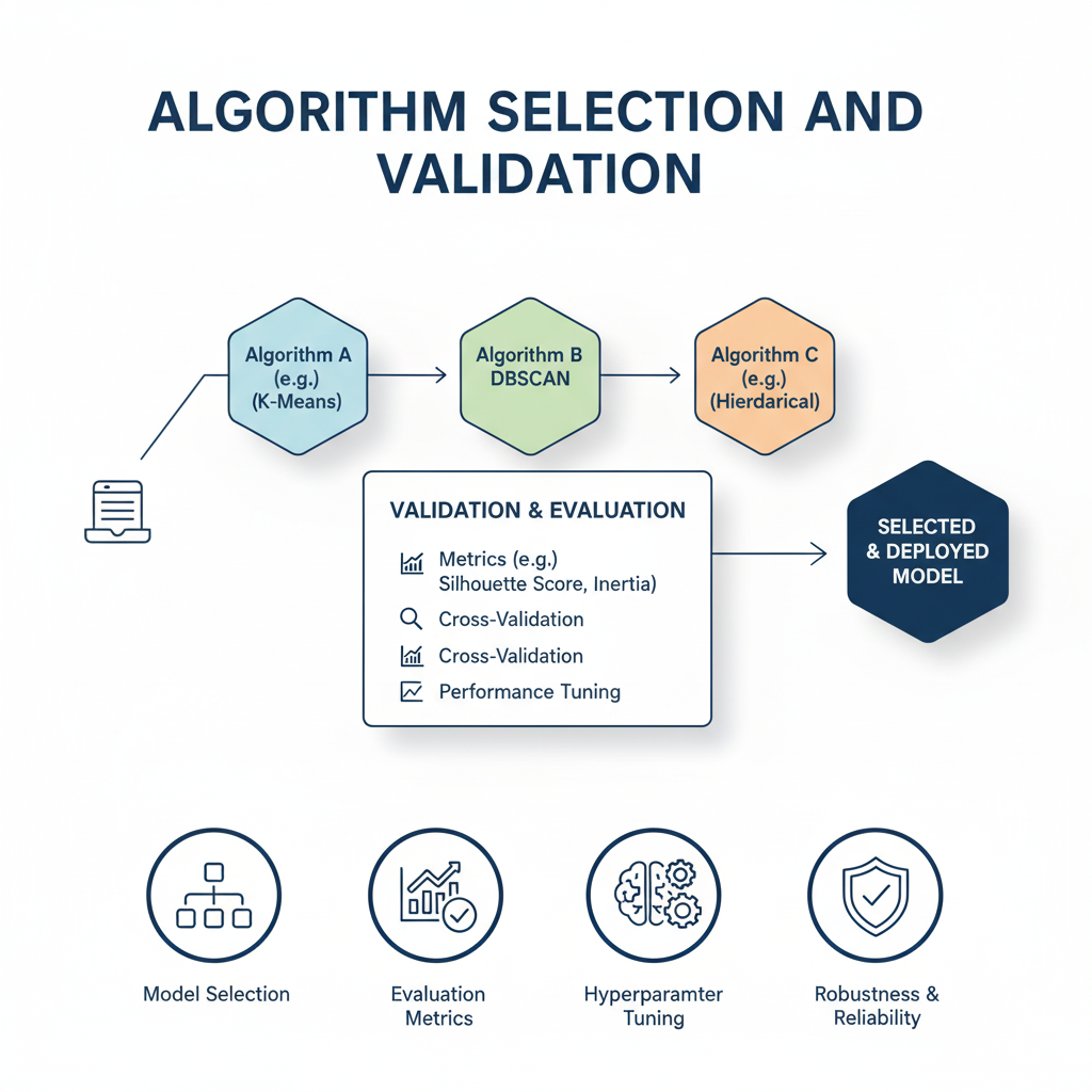
- Multi-Algorithm Evaluation: Test multiple clustering approaches with different parameter settings
- Stability Analysis: Assess cluster consistency across different random seeds and data samples
- Validation Framework:
- Internal Validation: Silhouette score, Davies-Bouldin index, Calinski-Harabasz index
- External Validation: Adjusted Rand index, normalized mutual information (when labels available)
- Visual Validation: t-SNE and UMAP projections for qualitative assessment
Phase 4: Interpretation and Actionable Insight Generation
- Cluster Profiling: Characterize each cluster using descriptive statistics and visualization
- Business Interpretation: Translate statistical clusters into meaningful segments or categories
- Action Planning: Develop specific strategies for each identified cluster
- Feedback Mechanisms: Establish processes for validating clusters with domain experts
7.2 Advanced Best Practices and Pitfall Avoidance
Handling High-Dimensional Data:
- Curse of Dimensionality Awareness: Understand that distance measures become less meaningful in very high dimensions
- Manifold Learning: Use techniques like UMAP or Isomap when data lies on a lower-dimensional manifold
- Subspace Clustering: Consider methods that can identify clusters in different feature subspaces
Dealing with Mixed Data Types:
- Custom Distance Metrics: Develop similarity measures that handle both numerical and categorical features
- Gower’s Distance: A popular choice for mixed-type data that standardizes different variable types
- Encoding Strategies: Use target encoding or entity embedding for categorical variables
Scalability and Computational Efficiency:
- Sampling Strategies: Use mini-batch approaches or data sampling for very large datasets
- Distributed Computing: Implement clustering algorithms using Spark MLlib or Dask for big data
- Incremental Clustering: Consider online clustering algorithms for streaming data scenarios
Robustness and Reproducibility:
- Multiple Initializations: Run algorithms with different random seeds to assess stability
- Ensemble Clustering: Combine results from multiple clustering methods for more robust solutions
- Version Control: Maintain detailed records of data preprocessing steps and algorithm parameters
Ethical Considerations and Bias Mitigation:
- Fairness Assessment: Evaluate whether clustering results disproportionately impact protected groups
- Transparency: Document limitations and assumptions of the clustering approach
- Human Oversight: Maintain expert review processes for critical applications
7.3 Operationalization and Continuous Improvement
Production Deployment:
- Monitoring Systems: Track cluster stability and quality over time
- Automated Retraining: Establish triggers for model retraining based on data drift detection
- Performance Dashboards: Create visualization tools for business users to monitor cluster evolution
Feedback Integration:
- Human-in-the-Loop Systems: Incorporate expert feedback to refine cluster definitions
- A/B Testing Framework: Validate the business impact of cluster-based interventions
- Iterative Refinement: Treat clustering as an iterative process rather than a one-time analysis
By following this comprehensive framework and adhering to these best practices, organizations can move beyond academic clustering exercises to build robust, production-ready clustering systems that deliver sustained business value. The key to success lies in balancing statistical rigor with practical business relevance, ensuring that clustering insights translate into actionable strategies and measurable outcomes.
Conclusion: Clustering as a Lens for Discovery
Clustering is more than a set of algorithms; it is a powerful paradigm for exploratory data analysis. It provides a lens through which we can look at unstructured, unlabeled data and find the patterns that lie beneath the surface. Understanding the fundamental philosophies behind algorithms like K-Means and DBSCAN empowers you to choose the right lens for the job.
K-Means offers a simple, efficient way to partition data when you have an idea of the number of groups. DBSCAN provides a more nuanced, robust approach for discovering the natural, often messy, structure of real-world data. By mastering these tools and the workflow that surrounds them, you transform from someone who merely analyzes data into someone who truly discovers its hidden stories.