Transformers Explained: Unlocking the Magic Behind ChatGPT and BERT in 2025

Introduction: The Architectural Revolution That Changed AI Forever

In the landscape of 2025’s artificial intelligence, a single architectural blueprint powers everything from the conversational fluency of ChatGPT to the deep language understanding of BERT, and from real-time language translation to generative video creation. This foundational architecture is the Transformer.

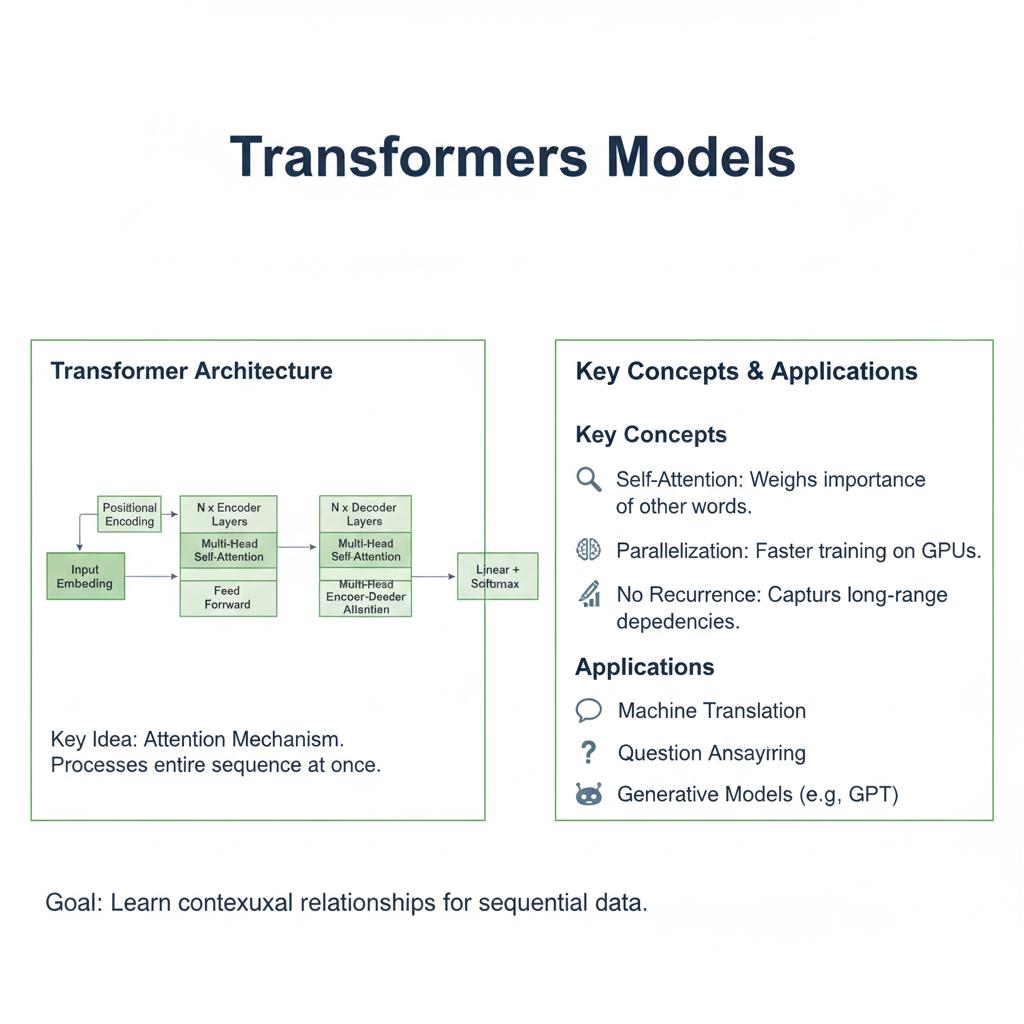
Introduced in the seminal 2017 paper “Attention Is All You Need” by Vaswani et al., the Transformer represents a fundamental paradigm shift in how we process sequential data. It completely abandoned the recurrent and convolutional layers that had previously dominated fields like natural language processing (NLP). Instead, it introduced a mechanism of self-attention, which allows the model to weigh the importance of all words in a sentence when processing any single word, regardless of their positional distance.

The impact of this innovation cannot be overstated. Before Transformers, models like RNNs and LSTMs processed data sequentially, creating a bottleneck that limited parallelization and made learning long-range dependencies difficult. Transformers process all elements of a sequence simultaneously, unlocking unprecedented scalability on modern hardware like GPUs and TPUs. This scalability directly enabled the era of Large Language Models (LLMs) that define the current AI frontier.

This article will deconstruct the magic behind Transformers. We will explore the core concepts of self-attention, walk through the architecture piece by piece, and demonstrate with practical code how this revolutionary model works. By the end, you will understand not just how Transformers power the AI tools you use every day, but also how to leverage them for your own applications.

Part 1: The Core Problem – The Limitations of Pre-Transformer Architectures

To appreciate the Transformer, we must first understand the limitations it overcame.

1.1 The Sequential Bottleneck of RNNs and LSTMs

Recurrent Neural Networks (RNNs) and their more sophisticated variant, Long Short-Term Memory networks (LSTMs), process data sequentially. To understand the meaning of the tenth word in a sentence, an RNN must process the first nine words one after another. This creates two major problems:

1. Lack of Parallelization: The sequential nature prevents parallel processing, making training on large datasets slow and computationally expensive.
2. Information Dilution: Although LSTMs mitigate the “vanishing gradient” problem, information can still become diluted or distorted when traveling over very long sequences. The context from the beginning of a long document may be lost by the end.

1.2 The Local Focus of CNNs

Convolutional Neural Networks (CNNs) can process data in parallel, but they primarily capture local relationships. A convolution operation with a 3×3 kernel can only see a small window of the input at a time. Capturing long-range dependencies requires many stacked layers, which is inefficient and can still fail for very long sequences.

The Transformer was designed to solve these problems by offering a mechanism that is both fully parallelizable and capable of directly connecting any two positions in the sequence, no matter how far apart they are.

Part 2: The Heart of the Transformer – Self-Attention Explained

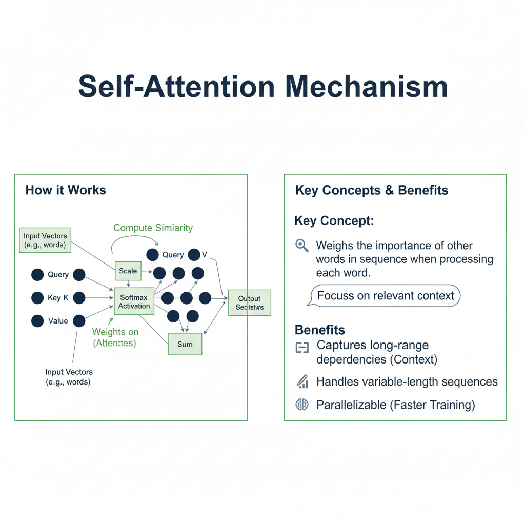
The self-attention mechanism is the revolutionary idea that makes the Transformer so powerful. It allows the model to look at every other word in the sentence when encoding a specific word.

2.1 The Intuition: “When I process this word, which other words should I pay attention to?”

Consider the sentence: “The animal didn’t cross the street because it was too tired.”

A human understands that “it” refers to “animal.” A simple model might struggle with this. Self-attention allows the Transformer to assign a high “attention score” between “it” and “animal,” effectively linking them directly. It does this for every word in the sentence, creating a rich, interconnected web of relationships.

2.2 The Mechanism: Queries, Keys, and Values

The self-attention mechanism is elegantly framed as a retrieval system. For each word (or “token”) in the input sequence, we create three vectors:

• Query (Q): “What am I looking for?” This vector represents the current word and is used to score against all other words.
• Key (K): “What I can offer?” This vector acts as an identifier for a word. The Query of one word is compared against the Key of every word to determine the attention score.
• Value (V): “What information I actually contain.” This vector holds the actual content of the word that will be propagated forward.

The process works as follows:

1. Calculate Attention Scores: For each word, we take its Query vector and compute a dot product with the Key vector of every word in the sentence (including itself). This results in a score indicating how much focus to place on other parts of the sentence when encoding the current word.
2. Scale and Softmax: The scores are scaled down (to prevent gradients from vanishing) and then passed through a softmax function. This normalizes the scores so they are all positive and sum to 1, creating a probability distribution—the “attention weights.”
3. Compute Output: The output for each word is a weighted sum of all the Value vectors, where the weights are the attention weights calculated in the previous step.

In essence, the self-attention layer allows every position in the sequence to directly “attend to” and incorporate information from every other position.

python

import tensorflow as tf
import numpy as np

def scaled_dot_product_attention(query, key, value, mask=None):
    """Calculate the attention weights and output."""
    # 1. Compute the raw attention scores: (batch_size, num_heads, seq_len_q, seq_len_k)
    matmul_qk = tf.matmul(query, key, transpose_b=True)

    # 2. Scale the scores
    depth = tf.cast(tf.shape(key)[-1], tf.float32)
    logits = matmul_qk / tf.math.sqrt(depth)
#transformers
    # 3. Apply the mask (for preventing attention to padding tokens or future words)
    if mask is not None:
        logits += (mask * -1e9) # Add a large negative number to masked positions

    # 4. Softmax to get the attention weights
    attention_weights = tf.nn.softmax(logits, axis=-1)

    # 5. Multiply weights by Values to get the final output
    output = tf.matmul(attention_weights, value)

    return output, attention_weights

# Example with a simple sequence
batch_size = 1
seq_len = 4
d_model = 64 # Dimension of the embedding space
#transformers
# Randomly initialize Q, K, V for 4 words, each with 64-dimensional embeddings
query = tf.random.normal((batch_size, seq_len, d_model))
key = tf.random.normal((batch_size, seq_len, d_model))
value = tf.random.normal((batch_size, seq_len, d_model))

output, attention_weights = scaled_dot_product_attention(query, key, value)

print(f"Input sequence length: {seq_len}")
print(f"Embedding dimension: {d_model}")
print(f"Output shape: {output.shape}") # (1, 4, 64)
print(f"Attention weights shape: {attention_weights.shape}") # (1, 4, 4)
print("\nAttention Matrix (showing how much each word attends to others):")
print(attention_weights[0].numpy())

Part 3: Building the Complete Transformer Architecture

Self-attention is the core, but the full Transformer architecture is a sophisticated system built around it. The original model uses an encoder-decoder structure, ideal for sequence-to-sequence tasks like translation.

3.1 The Encoder Stack

The encoder’s job is to process the input sequence and build a rich, contextualized representation. It consists of a stack of identical layers (the original paper used 6), each containing two main sub-layers:

1. Multi-Head Self-Attention: This is a supercharged version of the self-attention we just saw. Instead of performing a single attention function, the model linearly projects the Q, K, and V vectors into several different representation subspaces (“heads”) and performs attention in parallel. This allows the model to jointly attend to information from different perspectives (e.g., one head might focus on syntactic relationships, while another focuses on semantic meaning).
2. Position-wise Feed-Forward Network (FFN): This is a simple, fully connected neural network applied independently and identically to each position. It consists of two linear transformations with a ReLU (or Swish) activation in between. It allows for non-linear transformation of the representations produced by the attention layer.

Crucially, each of these sub-layers is surrounded by a residual connection and followed by layer normalization. This helps stabilize and accelerate the training of very deep networks.

3.2 The Decoder Stack

The decoder generates the output sequence (e.g., the translated sentence) one token at a time. It also consists of a stack of identical layers, but with three sub-layers:

1. Masked Multi-Head Self-Attention: This is a crucial difference. The decoder must be prevented from “peeking” at future tokens during training. A look-ahead mask ensures that when predicting a token at position i, the model can only attend to tokens at positions less than i.
2. Encoder-Decoder Attention: This is where the decoder “listens” to the encoder. The Queries for this layer come from the decoder’s previous layer, while the Keys and Values come from the output of the encoder stack. This allows every position in the decoder to attend over all positions in the input sequence.
3. Position-wise Feed-Forward Network: The same as in the encoder.

3.3 Positional Encoding: Injecting a Sense of Order

Since the Transformer contains no recurrence or convolution, it has no inherent notion of word order. To remedy this, positional encodings are added to the input embeddings. These encodings use a clever mix of sine and cosine functions of different frequencies to give the model information about the absolute and relative position of each token.

python

class TransformerBlock(tf.keras.layers.Layer):
    """A single Transformer encoder layer."""
    def __init__(self, d_model, num_heads, dff, dropout_rate=0.1):
        super(TransformerBlock, self).__init__()

        self.mha = tf.keras.layers.MultiHeadAttention(
            num_heads=num_heads, key_dim=d_model, dropout=dropout_rate
        )
        self.ffn = tf.keras.Sequential([
            tf.keras.layers.Dense(dff, activation='swish'),  # Position-wise FFN
            tf.keras.layers.Dense(d_model),
        ])

        self.layernorm1 = tf.keras.layers.LayerNormalization(epsilon=1e-6)
        self.layernorm2 = tf.keras.layers.LayerNormalization(epsilon=1e-6)
        self.dropout1 = tf.keras.layers.Dropout(dropout_rate)
        self.dropout2 = tf.keras.layers.Dropout(dropout_rate)

    def call(self, x, training, mask=None):
        # 1. Multi-Head Attention sub-layer
        attn_output = self.mha(query=x, value=x, key=x, attention_mask=mask, training=training)
        attn_output = self.dropout1(attn_output, training=training)
        out1 = self.layernorm1(x + attn_output)  # Residual connection + LayerNorm

        # 2. Feed-Forward Network sub-layer
        ffn_output = self.ffn(out1)
        ffn_output = self.dropout2(ffn_output, training=training)
        out2 = self.layernorm2(out1 + ffn_output)  # Another residual connection + LayerNorm

        return out2

class PositionalEncoding(tf.keras.layers.Layer):
    """Adds positional encoding to the input embeddings as described in the paper."""
    def __init__(self, position, d_model):
        super(PositionalEncoding, self).__init__()
        self.pos_encoding = self.positional_encoding(position, d_model)

    def get_angles(self, position, i, d_model):
        angles = 1 / tf.pow(10000, (2 * (i // 2)) / tf.cast(d_model, tf.float32))
        return position * angles

    def positional_encoding(self, position, d_model):
        angle_rads = self.get_angles(
            position=tf.range(position, dtype=tf.float32)[:, tf.newaxis],
            i=tf.range(d_model, dtype=tf.float32)[tf.newaxis, :],
            d_model=d_model
        )
        # apply sin to even indices in the array; 2i
        sines = tf.math.sin(angle_rads[:, 0::2])
        # apply cos to odd indices in the array; 2i+1
        cosines = tf.math.cos(angle_rads[:, 1::2])

        pos_encoding = tf.concat([sines, cosines], axis=-1)
        pos_encoding = pos_encoding[tf.newaxis, ...]
        return tf.cast(pos_encoding, tf.float32)

    def call(self, inputs):
        return inputs + self.pos_encoding[:, :tf.shape(inputs)[1], :]

# Build a small Transformer Encoder for demonstration
def build_transformer_encoder(vocab_size, num_layers, d_model, num_heads, dff, maximum_position_encoding, dropout_rate=0.1):
    inputs = tf.keras.layers.Input(shape=(None,), dtype=tf.int32)
    
    # Embedding Layer
    embedding = tf.keras.layers.Embedding(vocab_size, d_model)(inputs)
    
    # Positional Encoding
    positional_encoding = PositionalEncoding(maximum_position_encoding, d_model)
    x = positional_encoding(embedding)
    x = tf.keras.layers.Dropout(dropout_rate)(x)

    # Stack of Transformer Blocks
    for _ in range(num_layers):
        x = TransformerBlock(d_model, num_heads, dff, dropout_rate)(x)

    # The output of the encoder is the contextualized representation of the input
    model = tf.keras.Model(inputs=inputs, outputs=x)
    return model

# Example: Build a tiny encoder
vocab_size = 10000
num_layers = 2
d_model = 128
num_heads = 8
dff = 512
max_seq_length = 100

encoder = build_transformer_encoder(vocab_size, num_layers, d_model, num_heads, dff, max_seq_length)
encoder.summary()

Part 4: How Transformers Power ChatGPT and BERT

While the original Transformer was designed for sequence-to-sequence tasks, its architecture has been adapted to create the two main classes of models that dominate 2025: autoregressive models (like GPT and ChatGPT) and autoencoding models (like BERT).

4.1 The GPT / ChatGPT Family: Autoregressive Decoders

Models like ChatGPT are built using only the decoder part of the original Transformer. The key modification is that the self-attention in the decoder is masked, preventing the model from seeing future tokens. This architecture is called autoregressive.

• How it works: The model is trained to predict the next word in a sequence. Given the prompt “The weather is…”, it will generate a probability distribution over all possible next words (e.g., “nice,” “sunny,” “terrible”). It then samples a word, appends it to the sequence, and repeats the process to generate the next word. This creates the fluid, generative text we see in ChatGPT.
• Training: It’s trained on a massive corpus of internet text with a simple objective: “Given these N words, predict the N+1-th word.”

4.2 The BERT Family: Autoencoding Encoders

BERT (Bidirectional Encoder Representations from Transformers) uses only the encoder part of the original Transformer. Crucially, it does not use a causal mask, allowing it to see the entire input sequence bidirectionally.

• How it works: BERT is pre-trained using two main tasks:
  1. Masked Language Modeling (MLM): Random words in the input are masked (replaced with a [MASK] token), and the model is trained to predict the original word. This forces it to understand deep, bidirectional context.
  2. Next Sentence Prediction (NSP): The model is given two sentences and must predict if the second sentence logically follows the first.
• Fine-tuning: After this powerful pre-training, BERT can be fine-tuned with a simple classification layer on top for specific tasks like sentiment analysis, question answering, or named entity recognition.

Part 5: A Practical Walkthrough – Building a Sentiment Classifier with a Transformer Encoder

Let’s build a modern text classifier in 2025 using a Transformer encoder, similar to a simplified BERT, for sentiment analysis.

python

import tensorflow as tf
from tensorflow.keras import layers, Model
import tensorflow_datasets as tfds
#transformers
# Load the IMDB reviews dataset
(train_ds, test_ds), info = tfds.load('imdb_reviews', split=['train', 'test'], with_info=True, as_supervised=True)

# Prepare a TensorFlow Text vectorization layer
VOCAB_SIZE = 20000
MAX_SEQUENCE_LENGTH = 128

vectorize_layer = tf.keras.layers.TextVectorization(
    max_tokens=VOCAB_SIZE,
    output_mode='int',
    output_sequence_length=MAX_SEQUENCE_LENGTH
)

# Adapt the vectorization layer to the training data
train_text = train_ds.map(lambda text, label: text)
vectorize_layer.adapt(train_text)

def build_sentiment_transformer(vocab_size, max_length, d_model=128, num_heads=8, dff=512, num_layers=4):
    """Builds a BERT-like sentiment classifier using Transformer encoders."""
    
    # Input layer
    inputs = tf.keras.layers.Input(shape=(), dtype=tf.string, name='text_input')
    
    # Vectorization
    x = vectorize_layer(inputs)
    
    # Embedding Layer (Token + Positional)
    token_embedding = tf.keras.layers.Embedding(vocab_size, d_model, mask_zero=True)(x)
    #transformers
    # Positional Encoding (learned instead of fixed sine/cos)
    positions = tf.range(start=0, limit=max_length, delta=1)
    positions = tf.expand_dims(positions, axis=0)  # Add batch dimension
    positional_embedding = tf.keras.layers.Embedding(max_length, d_model)(positions)
    
    # Combine token and positional embeddings
    x = token_embedding + positional_embedding
    x = tf.keras.layers.Dropout(0.1)(x)
    
    # Stack of Transformer Encoder Layers
    for i in range(num_layers):
        x = TransformerBlock(d_model, num_heads, dff, dropout_rate=0.1)(x)
    
    # Classification Head
    # Use the [CLS] token equivalent (first token's representation)
    cls_token = x[:, 0, :]
    
    # Additional layers for classification
    x = tf.keras.layers.Dense(64, activation='swish')(cls_token)
    x = tf.keras.layers.Dropout(0.2)(x)
    outputs = tf.keras.layers.Dense(1, activation='sigmoid', name='classifier')(x)
    
    model = tf.keras.Model(inputs=inputs, outputs=outputs)
    return model

# Build and compile the model
model = build_sentiment_transformer(VOCAB_SIZE, MAX_SEQUENCE_LENGTH)
#transformers
model.compile(
    optimizer=tf.keras.optimizers.AdamW(learning_rate=2e-5, weight_decay=1e-4),
    loss='binary_crossentropy',
    metrics=['accuracy']
)

model.summary()

# Prepare the datasets
def prepare_dataset(ds):
    return ds.batch(32).prefetch(tf.data.AUTOTUNE)

train_ds_prepared = prepare_dataset(train_ds)
test_ds_prepared = prepare_dataset(test_ds)

# Train the model
print("Training the Transformer-based sentiment classifier...")
history = model.fit(
    train_ds_prepared,
    validation_data=test_ds_prepared,
    epochs=5,
    verbose=1
)

# Evaluate the model
test_loss, test_accuracy = model.evaluate(test_ds_prepared, verbose=0)
print(f"\nTest Accuracy: {test_accuracy:.4f}")

# Test with a sample review
sample_reviews = [
    "This movie was absolutely fantastic! The acting was superb and the plot was engaging from start to finish.",
    "A tedious and poorly written film with weak performances and a predictable storyline. Would not recommend.",
    "It was okay, nothing special but not terrible either. Some good moments but overall forgettable."
]
#transformers
predictions = model.predict(sample_reviews)
for review, pred in zip(sample_reviews, predictions):
    sentiment = "Positive" if pred > 0.5 else "Negative"
    confidence = pred[0] if pred > 0.5 else 1 - pred[0]
    print(f"\nReview: {review[:80]}...")
    print(f"Sentiment: {sentiment} (Confidence: {confidence:.2f})")

Part 6: The 2025 Landscape – Beyond NLP: Vision Transformers and Multimodal Models

The Transformer‘s success is no longer confined to language. Its ability to model relationships between elements has made it a versatile architecture across domains.

6.1 Vision Transformers (ViTs)

Vision Transformers apply the Transformer architecture directly to images. An image is split into fixed-size patches, linearly embedded, and then treated as a sequence of tokens, just like words in a sentence. Positional encodings are added to retain spatial information.

python

class VisionTransformer(tf.keras.Model):
    """A simplified Vision Transformer (ViT) for image classification."""
    def __init__(self, image_size=224, patch_size=16, num_layers=6, d_model=768, num_heads=12, dff=3072, num_classes=1000):
        super(VisionTransformer, self).__init__()
        #transformers
        self.patch_size = patch_size
        self.d_model = d_model
        self.num_patches = (image_size // patch_size) ** 2
        
        # Patch embedding layer
        self.patch_embed = tf.keras.layers.Conv2D(d_model, kernel_size=patch_size, strides=patch_size, padding='valid')
        self.flatten = tf.keras.layers.Reshape((self.num_patches, d_model))
        
        # Learnable [CLS] token for classification
        self.cls_token = self.add_weight(shape=(1, 1, d_model), initializer='random_normal', trainable=True, name='cls_token')
        
        # Positional embedding
        self.pos_embed = self.add_weight(shape=(1, self.num_patches + 1, d_model), initializer='random_normal', trainable=True, name='pos_embed')
        
        # Transformer encoder layers
        self.transformer_layers = [TransformerBlock(d_model, num_heads, dff) for _ in range(num_layers)]
        
        # Classification head
        self.layer_norm = tf.keras.layers.LayerNormalization(epsilon=1e-6)
        self.classifier = tf.keras.layers.Dense(num_classes, activation='softmax')
        
    def call(self, inputs, training=False):
        batch_size = tf.shape(inputs)[0]
        #transformers
        # Create patch embeddings
        patches = self.patch_embed(inputs)  # (batch, height/patch, width/patch, d_model)
        patches = self.flatten(patches)     # (batch, num_patches, d_model)
        
        # Prepend [CLS] token
        cls_tokens = tf.tile(self.cls_token, [batch_size, 1, 1])
        x = tf.concat([cls_tokens, patches], axis=1)  # (batch, num_patches + 1, d_model)
        
        # Add positional embeddings
        x += self.pos_embed
        
        # Apply transformer layers
        for transformer_layer in self.transformer_layers:
            x = transformer_layer(x, training=training)
        
        # Use the [CLS] token for classification
        x = self.layer_norm(x)
        cls_output = x[:, 0, :]  # Take the [CLS] token representation
        return self.classifier(cls_output)

6.2 Multimodal Transformers

The most exciting frontier in 2025 is multimodal Transformers, which can process and relate information from different modalities (text, image, audio) simultaneously. Models like DALL-E, Stable Diffusion, and GPT-4V are built on this principle, using Transformers to create a shared understanding across different types of data.

Conclusion: The Transformative Legacy

The Transformer architecture has proven to be one of the most consequential innovations in the history of artificial intelligence. Its core principles—self-attention, parallel processing, and scalability—have not only revolutionized natural language processing but have become a universal foundation for modern AI.

Understanding Transformers in 2025 is essential because:

• They are the fundamental building blocks of all major AI systems, from chatbots to code generators.
• Their architectural principles are domain-agnostic, applying equally well to language, vision, audio, and beyond.
• They enable the scale necessary for the large foundation models that are driving the current AI revolution.

The “magic” behind ChatGPT and BERT is not a mysterious black box but an elegant, well-understood architecture that excels at modeling relationships. By mastering the Transformer, you gain insight into the core engine of modern AI and equip yourself to build the intelligent systems of tomorrow. As we look beyond 2025, the principles of attention and contextual understanding pioneered by the Transformer will likely continue to shape the future of artificial intelligence for years to come.