Top 10 Feature Selection Techniques Every Data Scientist Should Know

Introduction: The “Curse of Dimensionality” and the Power of Feature Selection

In the era of big data, it’s tempting to throw every possible variable into a machine learning model, hoping it will find the signal in the noise. However, this approach often backfires, leading to a phenomenon known as the “Curse of Dimensionality.” As the number of features grows, the data becomes increasingly sparse, making it harder for models to learn effectively. This results in models that are slower, more complex, and prone to overfitting—performing well on training data but failing to generalize to new, unseen data.

This is where Feature Selection becomes not just useful, but essential. Feature Selection is the process of automatically or manually selecting the most relevant and informative subset of features from your original dataset for use in model construction. It is a critical step in the data preprocessing pipeline that directly addresses core data science principles.

The benefits of effective Feature Selection are profound:

• Reduces Overfitting: Less redundant data means less opportunity for the model to learn noise.
• Improves Model Performance: By eliminating irrelevant features, the model can focus on the true signals, often leading to higher accuracy.
• Enhances Training Speed: Fewer features mean fewer computations, drastically reducing model training time.
• Increases Model Interpretability: A simpler model with fewer features is easier to understand, explain, and trust, which is crucial for stakeholder buy-in and regulatory compliance.

This article will explore the top 10 Feature Selection techniques, categorized by their approach, that every data scientist should have in their toolkit. We will move from simple, intuitive methods to advanced, model-driven algorithms, complete with practical Python examples.

Part 1: The Three Paradigms of Feature Selection

Before diving into the techniques, it’s crucial to understand the three main families of Feature Selection methods:

1. Filter Methods: These methods select features based on their intrinsic statistical properties, independent of any machine learning model. They are generally fast and scalable but may ignore feature dependencies.
2. Wrapper Methods: These methods use a specific machine learning model to evaluate the quality of feature subsets. They perform a search for a high-performing subset of features, making them computationally expensive but often very effective.
3. Embedded Methods: These methods perform Feature Selection as part of the model construction process itself. They offer a trade-off between the computational efficiency of filter methods and the performance of wrapper methods.

The following top 10 list is organized within this framework.

Category 1: Filter Methods

1. Correlation-Based Feature Selection

Idea: Remove features that are highly correlated with each other. If two features convey the same information, one is redundant.

How it works: A correlation matrix (e.g., Pearson’s for linear relationships) is calculated. For each pair of highly correlated features (above a defined threshold, e.g., 0.9), one is removed.

When to use: As a quick, first-pass cleanup, especially when you suspect multicollinearity in linear models.

Python Example:

python

import pandas as pd
import numpy as np
import seaborn as sns
import matplotlib.pyplot as plt

# Calculate correlation matrix
corr_matrix = df.corr().abs()

# Create a mask for the upper triangle
upper_tri = corr_matrix.where(np.triu(np.ones_like(corr_matrix, dtype=bool), k=1))

# Find features with correlation greater than 0.95
to_drop = [column for column in upper_tri.columns if any(upper_tri[column] > 0.95)]

# Drop the features
df_reduced = df.drop(to_drop, axis=1)
print(f"Dropped {len(to_drop)} features: {to_drop}")

2. Univariate Feature Selection (Chi-Squared, ANOVA F-test)

Idea: Select the best features based on univariate statistical tests that evaluate the relationship between each feature and the target variable.

How it works:

• For Classification: SelectKBest with chi2 (for categorical features) or f_classif (for numerical features).
• For Regression: SelectKBest with f_regression or mutual_info_regression.

These tests score each feature independently, and you select the top K features.

When to use: A very fast and scalable method to reduce a very large feature space to a manageable number before applying more sophisticated methods.

Python Example:

python

from sklearn.feature_selection import SelectKBest, f_classif
from sklearn.datasets import load_breast_cancer

# Load dataset
data = load_breast_cancer()
X, y = data.data, data.target

# Apply SelectKBest to get the top 10 features
selector = SelectKBest(score_func=f_classif, k=10)
X_new = selector.fit_transform(X, y)

# Get the selected feature names
selected_features = data.feature_names[selector.get_support()]
print("Top 10 features:", selected_features)

3. Variance Threshold

Idea: Remove features with low variance, as they contain little to no information.

How it works: It simply removes all features whose variance doesn’t meet a certain threshold. By default, it removes zero-variance features (features that have the same value in all samples).

When to use: An excellent baseline Feature Selection method to remove constant and quasi-constant features.

Python Example:

python

from sklearn.feature_selection import VarianceThreshold

# Initialize selector to remove features with >80% similar values
selector = VarianceThreshold(threshold=(.8 * (1 - .8)))
X_reduced = selector.fit_transform(X)

print(f"Original shape: {X.shape}")
print(f"Reduced shape: {X_reduced.shape}")

4. Mutual Information

Idea: Measures the dependency between two variables. It can capture any kind of relationship, linear or non-linear, making it more powerful than correlation.

How it works: It quantifies the amount of information obtained about one random variable through the other random variable. A higher score indicates a stronger dependency.

When to use: When you suspect complex, non-linear relationships between features and the target.

Python Example:

python

from sklearn.feature_selection import SelectKBest, mutual_info_classif

# Select top 10 features based on Mutual Information
mi_selector = SelectKBest(score_func=mutual_info_classif, k=10)
X_mi = mi_selector.fit_transform(X, y)

# Get scores for all features
mi_scores = mutual_info_classif(X, y)
mi_scores = pd.Series(mi_scores, index=data.feature_names)
mi_scores.sort_values(ascending=False).plot.bar(figsize=(10, 5))
plt.title("Mutual Information Scores")

Category 2: Wrapper Methods

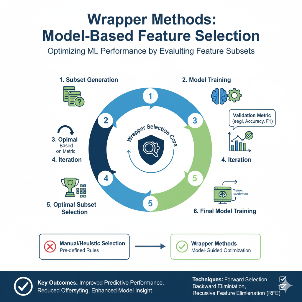
5. Recursive Feature Elimination (RFE)

Idea: Recursively removes the least important features, building a model on the remaining features until the desired number of features is reached.

How it works:

1. Train a model (e.g., a linear model or decision tree) that can assign feature importance.
2. Discard the least important feature(s).
3. Re-train the model on the remaining features.
4. Repeat steps 2-3 until the predefined number of features is reached.

When to use: When you have a medium-sized dataset and want a robust, model-aware selection process.

Python Example:

python

from sklearn.feature_selection import RFE
from sklearn.linear_model import LogisticRegression
from sklearn.datasets import load_breast_cancer

data = load_breast_cancer()
X, y = data.data, data.target

# Create a base model
model = LogisticRegression(solver='liblinear', max_iter=1000)

# Initialize RFE to select 10 features
rfe = RFE(estimator=model, n_features_to_select=10)
X_rfe = rfe.fit_transform(X, y)

print("Selected features:", data.feature_names[rfe.get_support()])
print("Feature Rankings (1 is best):", rfe.ranking_)

6. Sequential Feature Selector (Forward/Backward Selection)

Idea: A greedy search algorithm that builds the feature subset step-by-step.

• Forward Selection: Starts with no features and adds one feature at a time that most improves the model until no significant improvement is seen.
• Backward Elimination: Starts with all features and removes one feature at a time that least hurts the model until no significant improvement is seen from removal.

When to use: When you want a thorough search and computational cost is not a primary concern. It often finds a very good feature subset.

Python Example (using mlxtend):

python

# pip install mlxtend
from mlxtend.feature_selection import SequentialFeatureSelector as SFS
from sklearn.ensemble import RandomForestClassifier

# Create a Random Forest model
rf = RandomForestClassifier(n_estimators=10, random_state=42)

# Perform Forward Selection
sfs = SFS(rf,
          k_features=10,
          forward=True,
          floating=False,
          scoring='accuracy',
          cv=5,
          n_jobs=-1)

sfs = sfs.fit(X, y)

# Print the results
print(f"Best accuracy score: {sfs.k_score_:.4f}")
print("Best feature subset:", sfs.k_feature_names_)

Category 3: Embedded Methods

7. Lasso (L1 Regularization) Regression

Idea: A regularization technique that adds a penalty equal to the absolute value of the magnitude of coefficients. This penalty has the effect of forcing some coefficients to be exactly zero, effectively performing Feature Selection.

How it works: The L1 penalty shrinks coefficients, and for less important features, it drives them all the way to zero. Any feature with a non-zero coefficient is considered “selected.”

When to use: Primarily for linear models when you want both regularization and Feature Selection. Excellent for dealing with high-dimensional data.

Python Example:

python

from sklearn.linear_model import LassoCV
from sklearn.preprocessing import StandardScaler

# It's crucial to standardize data for Lasso
scaler = StandardScaler()
X_scaled = scaler.fit_transform(X)

# Use LassoCV to find the best alpha (regularization strength) via cross-validation
lasso = LassoCV(cv=5, random_state=42, max_iter=10000).fit(X_scaled, y)

# Get the coefficients
coef = pd.Series(lasso.coef_, index=data.feature_names)

# Selected features are those with non-zero coefficients
selected_features = coef[coef != 0].index
print(f"Lasso selected {len(selected_features)} features:")
print(selected_features.tolist())

# Plot the coefficients
imp_coef = coef.sort_values()
plt.figure(figsize=(10, 6))
imp_coef.plot(kind='barh')
plt.title("Feature importance using Lasso")
plt.show()

8. Tree-Based Feature Importance

Idea: Tree-based algorithms (like Random Forest and Gradient Boosting) naturally provide a measure of feature importance based on how much a feature decreases the impurity (Gini impurity or entropy for classification, MSE for regression) across all trees.

How it works: The importance of a feature is computed as the (normalized) total reduction of the impurity criterion brought by that feature.

When to use: Anytime you are using or considering tree-based models. It’s a fast and powerful way to get feature importance scores.

Python Example:

python

from sklearn.ensemble import RandomForestClassifier

# Train a Random Forest model
rf = RandomForestClassifier(n_estimators=100, random_state=42)
rf.fit(X, y)

# Get feature importances
importances = rf.feature_importances_
feature_imp = pd.Series(importances, index=data.feature_names).sort_values(ascending=False)

# Plot the top N features
top_n = 15
plt.figure(figsize=(10, 6))
feature_imp.head(top_n).plot(kind='barh')
plt.title(f"Top {top_n} Features from Random Forest")
plt.gca().invert_yaxis()
plt.show()

# Select features above a certain importance threshold
threshold = 0.01
selected_features = feature_imp[feature_imp > threshold].index
X_selected = df[selected_features]

9. Permutation Feature Importance

Idea: A model-agnostic technique that measures the importance of a feature by calculating the increase in the model’s prediction error after permuting the feature’s values. If a feature is important, shuffling its values should significantly decrease the model’s performance.

How it works:

1. Train a model and record a baseline score (e.g., R² for regression).
2. For each feature, shuffle its values and recalculate the model’s score.
3. The importance of the feature is the drop in performance from the baseline.

When to use: When you want a robust, model-agnostic measure of feature importance that is reliable for any model.

Python Example:

python

from sklearn.inspection import permutation_importance
from sklearn.model_selection import train_test_split

# Split the data
X_train, X_test, y_train, y_test = train_test_split(X, y, test_size=0.3, random_state=42)

# Train a model (could be any model)
model = RandomForestClassifier(n_estimators=100, random_state=42).fit(X_train, y_train)

# Calculate permutation importance
perm_importance = permutation_importance(model, X_test, y_test, n_repeats=10, random_state=42, n_jobs=-1)

# Organize and display results
sorted_idx = perm_importance.importances_mean.argsort()[::-1]
plt.figure(figsize=(10, 6))
plt.barh(np.array(data.feature_names)[sorted_idx][:15], perm_importance.importances_mean[sorted_idx][:15])
plt.xlabel("Permutation Importance")
plt.title("Top 15 Features by Permutation Importance")
plt.gca().invert_yaxis()
plt.show()

Category 4: Advanced / Hybrid Methods

10. Boruta

Idea: An all-relevant Feature Selection algorithm that finds all features that are in some circumstances relevant, not just the strongest ones. It’s a wrapper built around Random Forest.

How it works:

1. It creates “shadow features” by shuffling the original features (these represent noise).
2. It trains a Random Forest classifier on the extended dataset (original + shadow features).
3. It compares the importance of original features with the maximum importance of shadow features.
4. A feature is deemed “important” if it consistently performs better than the best shadow feature over multiple iterations.

When to use: When you want a highly robust method that tries to find all features that have any predictive power, not just the most obvious ones.

Python Example:

python

# pip install boruta
from boruta import BorutaPy
from sklearn.ensemble import RandomForestClassifier

# Define the model Boruta will use
rf = RandomForestClassifier(n_estimators='auto', max_depth=5, random_state=42, n_jobs=-1)

# Initialize Boruta
boruta_selector = BorutaPy(rf, n_estimators='auto', verbose=2, random_state=42, max_iter=100)

# Fit Boruta (it takes numpy arrays, not pandas DataFrames)
boruta_selector.fit(X, y)

# Get the results
print("\nBoruta Selection Results:")
print(f"Number of selected features: {boruta_selector.n_features_}")
print(f"Selected features mask: {boruta_selector.support_}")

# Get the selected feature names
selected_features = data.feature_names[boruta_selector.support_]
print("Features selected by Boruta:", selected_features)

Part 2: Building a Practical Feature Selection Workflow

Knowing individual techniques is not enough; a data scientist must know how to combine them into a coherent strategy.

A Recommended Multi-Stage Workflow:

1. Data Cleaning (Variance Threshold): Start by removing constant and quasi-constant features. They add no value.
2. Redundancy Removal (Correlation): Identify and remove highly correlated duplicate features to reduce multicollinearity.
3. Coarse Filtering (Univariate Selection): Use a fast filter method like SelectKBest with Mutual Information or ANOVA to reduce the feature space from hundreds to a few dozen.
4. Fine-Tuned Selection (Embedded/Wrapper): Apply a more sophisticated method like Lasso, Random Forest feature importance, or Boruta on the reduced feature set to get your final, robust subset.

Category 5: Modern and Hybrid Feature Selection Techniques

As machine learning evolves, new Feature Selection methods have emerged that combine multiple approaches or leverage modern computational frameworks to handle the scale and complexity of contemporary datasets.

11. Stability Selection with Randomized Lasso

Idea: A robust method that combines subsampling with Lasso regression to identify features that are consistently selected across different data perturbations.

How it works:

1. Multiple subsamples of the data are taken
2. Lasso regression is run on each subsample with randomized penalties
3. Features that are frequently selected across different subsamples are deemed stable
4. This method significantly reduces false positive selections

When to use: When working with high-dimensional data where traditional Lasso might be unstable, and you need more reliable feature selection.

Python Example:

python

from sklearn.linear_model import RandomizedLasso
from sklearn.datasets import load_breast_cancer
import numpy as np

# Load dataset
data = load_breast_cancer()
X, y = data.data, data.target

# Initialize Randomized Lasso
rlasso = RandomizedLasso(alpha=0.025, scaling=0.5, sample_fraction=0.75, 
                        n_resampling=200, random_state=42)
rlasso.fit(X, y)

# Get feature scores
scores = rlasso.scores_
feature_scores = pd.Series(scores, index=data.feature_names)
selected_features = feature_scores[feature_scores > 0.8].index

print(f"Stable features selected: {len(selected_features)}")
print("Selected features:", selected_features.tolist())

# Plot stability scores
plt.figure(figsize=(12, 6))
feature_scores.sort_values(ascending=False).plot.bar()
plt.axhline(y=0.8, color='r', linestyle='--', label='Stability Threshold')
plt.title('Stability Selection Scores')
plt.ylabel('Selection Probability')
plt.legend()
plt.show()

12. SHAP-based Feature Selection

Idea: Use SHapley Additive exPlanations (SHAP) values to select features based on their actual contribution to model predictions, providing a unified measure of feature importance across any model type.

How it works:

1. Train any machine learning model
2. Calculate SHAP values for all features
3. Aggregate SHAP values to get global feature importance
4. Select features with highest mean absolute SHAP values

When to use: When you need model-agnostic, theoretically sound feature importance that accounts for feature interactions.

Python Example:

python

import shap
from sklearn.ensemble import RandomForestClassifier
from sklearn.model_selection import train_test_split

# Split data
X_train, X_test, y_train, y_test = train_test_split(X, y, test_size=0.3, random_state=42)

# Train model
model = RandomForestClassifier(n_estimators=100, random_state=42)
model.fit(X_train, y_train)

# Calculate SHAP values
explainer = shap.TreeExplainer(model)
shap_values = explainer.shap_values(X_test)

# For classification, we typically look at one class
if isinstance(shap_values, list):
    shap_values = shap_values[1]  # Class 1 for binary classification

# Calculate mean absolute SHAP values for each feature
shap_importance = np.abs(shap_values).mean(0)
shap_series = pd.Series(shap_importance, index=data.feature_names).sort_values(ascending=False)

# Select top features based on SHAP importance
top_k = 10
selected_features = shap_series.head(top_k).index

print(f"Top {top_k} features by SHAP importance:")
for i, (feature, importance) in enumerate(shap_series.head(top_k).items(), 1):
    print(f"{i}. {feature}: {importance:.4f}")

# Create SHAP summary plot
shap.summary_plot(shap_values, X_test, feature_names=data.feature_names, show=False)
plt.tight_layout()
plt.show()

13. AutoML-based Feature Selection

Idea: Leverage Automated Machine Learning platforms that intrinsically perform feature selection as part of their optimization process.

How it works: AutoML systems like AutoSklearn, H2O.ai, and TPOT automatically explore different feature subsets along with model hyperparameters, using meta-learning and ensemble methods to find optimal combinations.

When to use: When you want an end-to-end solution that handles feature selection, model selection, and hyperparameter tuning simultaneously.

Python Example with TPOT:

python

from tpot import TPOTClassifier
from sklearn.model_selection import train_test_split
import numpy as np

# Split data
X_train, X_test, y_train, y_test = train_test_split(X, y, test_size=0.3, random_state=42)

# Initialize TPOT with feature selection emphasis
tpot = TPOTClassifier(
    generations=5,
    population_size=20,
    verbosity=2,
    random_state=42,
    config_dict='TPOT light',  # Faster configuration
    n_jobs=-1,
    scoring='accuracy'
)

# Fit TPOT - this will automatically perform feature selection
print("Starting AutoML feature selection with TPOT...")
tpot.fit(X_train, y_train)

# Evaluate the best pipeline
print(f"Best pipeline score: {tpot.score(X_test, y_test):.4f}")

# Export the best pipeline code to see what features were selected
tpot.export('best_pipeline_with_feature_selection.py')

# The exported Python file will show the exact preprocessing and feature selection steps

14. Deep Learning-based Feature Selection

Idea: Use neural networks with specific architectures designed for feature selection, such as autoencoders with sparsity constraints or attention mechanisms.

How it works:

• Autoencoders: Train an autoencoder and use the encoder weights to determine feature importance
• Attention Mechanisms: Use attention layers to learn feature importance weights
• Sparse Neural Networks: Apply L1 regularization to input layers to drive feature weights to zero

When to use: For very high-dimensional data (e.g., genomics, text) where traditional methods struggle, and when you’re already using deep learning.

Python Example with Sparse Autoencoder:

python

import tensorflow as tf
from tensorflow.keras import layers, models, regularizers
from sklearn.preprocessing import StandardScaler
import numpy as np

# Standardize the data
scaler = StandardScaler()
X_scaled = scaler.fit_transform(X)

# Build a sparse autoencoder for feature selection
input_dim = X_scaled.shape[1]
encoding_dim = 10  # Bottleneck layer size

# Input layer
input_layer = layers.Input(shape=(input_dim,))

# Encoder with L1 sparsity constraint
encoded = layers.Dense(64, activation='relu', 
                      activity_regularizer=regularizers.l1(10e-5))(input_layer)
encoded = layers.Dense(32, activation='relu', 
                      activity_regularizer=regularizers.l1(10e-5))(encoded)
bottleneck = layers.Dense(encoding_dim, activation='relu')(encoded)

# Decoder
decoded = layers.Dense(32, activation='relu')(bottleneck)
decoded = layers.Dense(64, activation='relu')(decoded)
output_layer = layers.Dense(input_dim, activation='linear')(decoded)

# Compile autoencoder
autoencoder = models.Model(input_layer, output_layer)
autoencoder.compile(optimizer='adam', loss='mse')

# Train autoencoder
history = autoencoder.fit(X_scaled, X_scaled,
                         epochs=100,
                         batch_size=32,
                         shuffle=True,
                         validation_split=0.2,
                         verbose=0)

# Extract encoder model
encoder = models.Model(input_layer, bottleneck)

# Get feature importance from first layer weights
first_layer_weights = autoencoder.layers[1].get_weights()[0]
feature_importance = np.abs(first_layer_weights).mean(axis=1)

# Create feature importance series
feature_importance_series = pd.Series(feature_importance, index=data.feature_names)
selected_features = feature_importance_series.nlargest(10).index

print("Top features selected by sparse autoencoder:")
print(selected_features.tolist())

15. Federated Feature Selection

Idea: Perform feature selection across distributed datasets without centralizing the data, preserving privacy while maintaining selection quality.

How it works:

1. Compute feature importance locally on each node
2. Aggregate importance scores centrally using secure protocols
3. Select features based on aggregated scores
4. This is particularly useful for healthcare, finance, and multi-institutional collaborations

When to use: When working with sensitive, distributed data across multiple locations or institutions where data cannot be pooled.

Python Conceptual Example:

python

import numpy as np
from typing import List, Dict
from sklearn.ensemble import RandomForestClassifier

class FederatedFeatureSelector:
    def __init__(self, n_features_to_select: int = 10):
        self.n_features_to_select = n_features_to_select
        self.global_feature_importance = None
    
    def compute_local_importance(self, X_local, y_local) -> Dict:
        """Compute feature importance on local data"""
        model = RandomForestClassifier(n_estimators=50, random_state=42)
        model.fit(X_local, y_local)
        
        local_importance = {
            'feature_scores': model.feature_importances_,
            'n_samples': len(X_local)
        }
        return local_importance
    
    def aggregate_importance(self, local_results: List[Dict]) -> np.array:
        """Aggregate feature importance across nodes"""
        total_samples = sum(result['n_samples'] for result in local_results)
        weighted_scores = np.zeros_like(local_results[0]['feature_scores'])
        
        for result in local_results:
            weight = result['n_samples'] / total_samples
            weighted_scores += result['feature_scores'] * weight
        
        return weighted_scores
    
    def select_features(self, local_datasets: List[tuple]) -> List[int]:
        """Main method to perform federated feature selection"""
        # Each node computes local importance
        local_importances = []
        for X_local, y_local in local_datasets:
            local_imp = self.compute_local_importance(X_local, y_local)
            local_importances.append(local_imp)
        
        # Aggregate importance scores
        self.global_feature_importance = self.aggregate_importance(local_importances)
        
        # Select top features
        top_feature_indices = np.argsort(self.global_feature_importance)[-self.n_features_to_select:]
        
        return sorted(top_feature_indices)

# Example usage with simulated distributed data
# In practice, this would run on different servers/nodes
federated_selector = FederatedFeatureSelector(n_features_to_select=8)

# Simulate 3 different data sources
local_datasets = [
    (X[:100], y[:100]),  # Node 1 data
    (X[100:200], y[100:200]),  # Node 2 data
    (X[200:], y[200:])  # Node 3 data
]

selected_features = federated_selector.select_features(local_datasets)
print(f"Federated selected features: {selected_features}")
print(f"Global feature importance: {federated_selector.global_feature_importance}")

Conclusion: Selecting Your Selector

There is no single “best” Feature Selection technique. The optimal choice depends on your dataset size, data types, model choice, and computational budget.

• For Speed: Start with Variance Threshold and Univariate Selection.
• For Robustness with Linear Models: Use Lasso Regression.
• For Tree-Based Models: Leverage built-in Tree-Based Feature Importance or Permutation Importance.
• For a Thorough, All-Relevant Search: Invest the computation in Boruta.
• For a General-Purpose, Model-Agnostic Pipeline: Combine Correlation Filtering with Recursive Feature Elimination (RFE).

Mastering these top 10 Feature Selection techniques will empower you to build models that are not only more accurate and efficient but also simpler and more interpretable. In a world where data is abundant but insight is precious, the ability to intelligently select the right features is what separates a good data scientist from a great one.