Master RNN in 2025 — Turn Data into Predictions with Deep Learning

Explore RNNs in 2025 — learn how Recurrent Neural Networks power AI, time series, and NLP with Python. Master sequence learning step-by-step.

Introduction: The Unfolding Power of Sequence Modeling

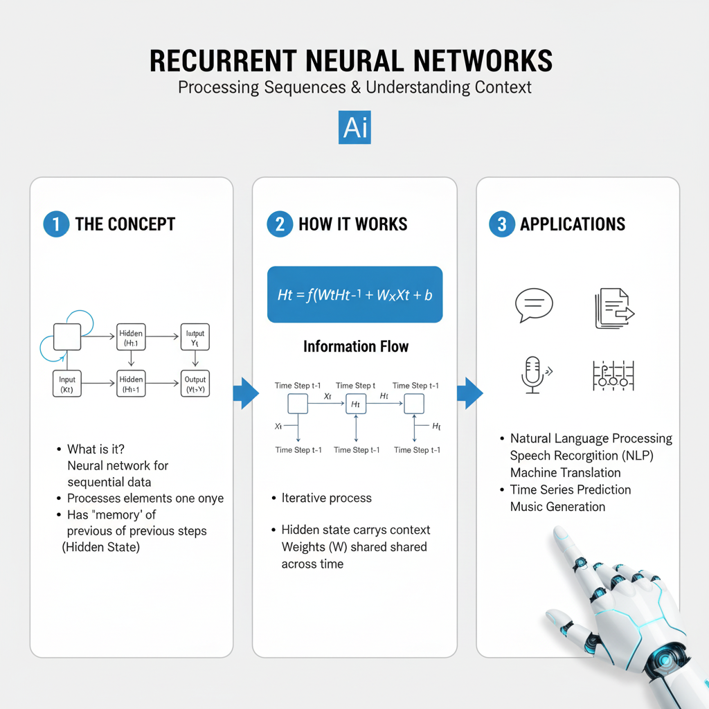
In a world increasingly governed by data that flows through time—from financial markets and sensor readings to human language and genomic sequences—the ability to understand and predict temporal patterns is a superpower. While other neural networks see the world in static snapshots, the Recurrent Neural Network, or RNN, perceives it as a dynamic, unfolding story. It is the foundational architecture designed to work with sequential data by maintaining a “memory” of previous information, allowing it to model time and order.

The narrative around RNNs in 2025 is one of sophisticated evolution, not obsolescence. Despite the rise of Transformers, RNNs and their advanced variants remain critically important. They offer a compelling blend of computational efficiency, strong performance on many tasks, and a fundamentally different approach to handling context that makes them ideal for streaming data, edge computing, and applications where low latency is paramount. Mastering the RNN family is essential for any data scientist looking to build intelligent systems that understand the dimension of time.

This guide will take you from the core concepts of recurrence to the advanced, modern implementations of RNN architectures. You will learn not only how they work but also how to apply them effectively in 2025’s ecosystem to turn streams of data into powerful, predictive insights.

Part 1: The Core Concept – Why Recurrence Matters

At its heart, an RNN is distinguished by a loop within its architecture. This loop allows information to persist, creating a bridge from the past to the present.

1.1 The Problem with Feedforward Networks

Standard neural networks (MLPs, CNNs) assume all inputs and outputs are independent of each other. They are stateless. This is a catastrophic assumption for sequential data. Consider predicting the next word in a sentence:

• Input: “The concert was so loud, my ears are still…”
• A feedforward network would struggle, as it has no memory that the subject was a “concert” or that it was “loud.”
• An , however, can use its internal state to remember the context, making “ringing” a highly probable prediction.

1.2 The RNN Loop: Unfolding in Time

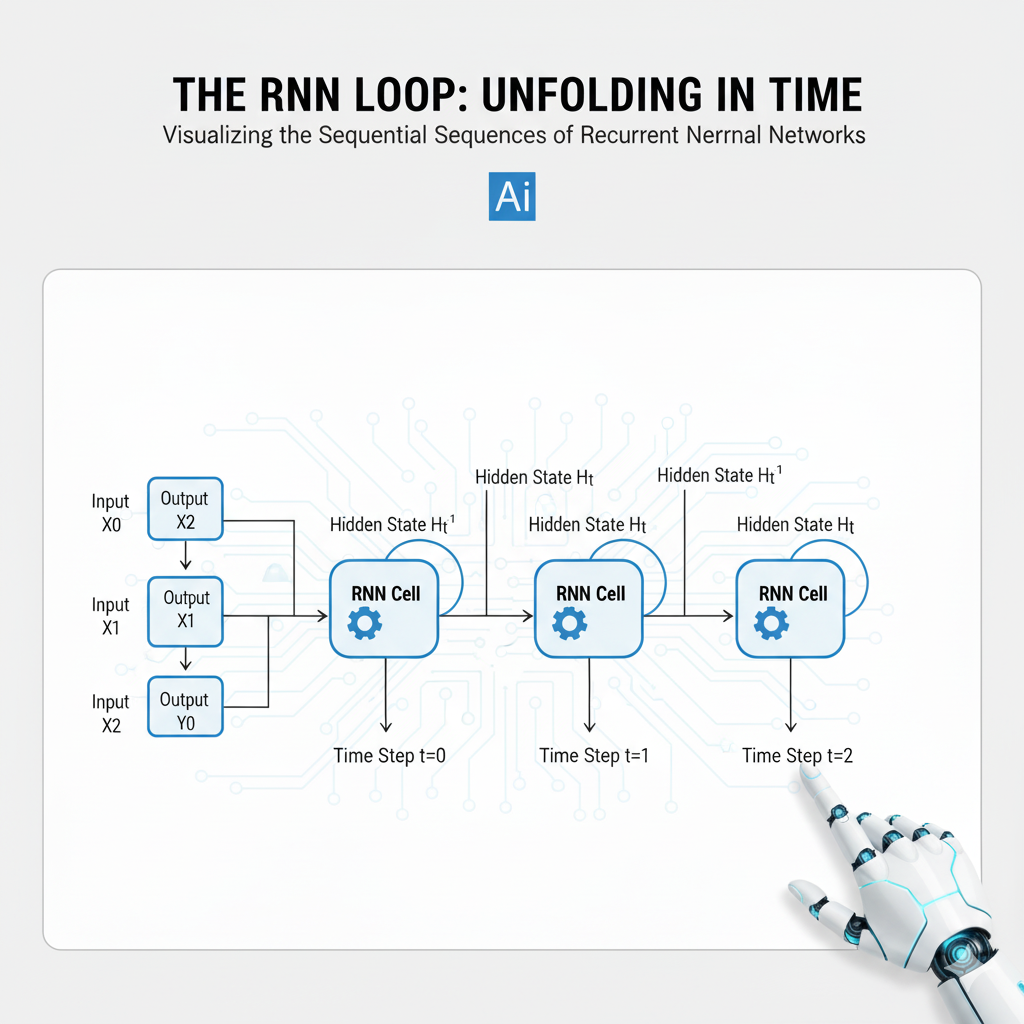
The magic of the RNN lies in its recurrent cell. At each time step t, the cell processes two inputs:

1. The current input, x_t (e.g., a word in a sentence, a stock price for a day).
2. A hidden state, h_{t-1}, which is a vector representing the network’s memory of all previous time steps.

It then produces two outputs:

1. An output for the current step, y_t (e.g., a prediction).
2. An updated hidden state, h_t, which is passed to the next time step.

This process can be visually “unfolded” into a deep network, where each layer corresponds to a moment in time. This reveals the fundamental challenge and the source of the  power: the ability to connect information across many time steps.

Part 2: The Vanishing Gradient Problem and The Rise of Gated Architectures

The simple or “vanilla” RNN has a critical flaw: it struggles to learn long-range dependencies. The core issue is the vanishing/exploding gradient problem.

The Problem Explained:
During training, gradients are calculated via backpropagation through time (BPTT). For a long sequence, this involves multiplying the same weight matrix repeatedly. If the eigenvalues of this matrix are less than 1, the gradient shrinks exponentially (vanishes). If they are greater than 1, it grows exponentially (explodes). A vanishing gradient means the early parts of a sequence have an negligible effect on learning, preventing the network from capturing context that spans many time steps.

This limitation led to the development of gated architectures, which introduced a more sophisticated memory system with mechanisms to selectively remember and forget information.

2.1 Long Short-Term Memory (LSTM): The Memory Cell

The LSTM, introduced in 1997, was a revolutionary solution. It introduces a separate cell state, C_t, which acts like a conveyor belt running through the entire sequence chain, with minor, linear interactions. Information is added or removed from this cell state via three regulatory gates:

• Forget Gate (f_t): Decides what information to throw away from the cell state. It looks at the previous hidden state h_{t-1} and the current input x_t, and outputs a number between 0 and 1 for each number in the cell state C_{t-1}.
• Input Gate (i_t): Decides what new information to store in the cell state. It has two parts: a sigmoid layer that decides which values to update, and a tanh layer that creates a vector of new candidate values, ~C_t.
• Output Gate (o_t): Decides what the next hidden state h_t should be. The hidden state is a filtered version of the cell state.

This gated architecture allows the LSTM to learn which information is relevant to keep or discard over long periods, making it exceptionally powerful for tasks like machine translation and speech recognition.

2.2 Gated Recurrent Unit (GRU): The Streamlined Alternative

The GRU, introduced in 2014, is a more recent and simplified variant of the LSTM. It combines the forget and input gates into a single “update gate.” It also merges the cell state and hidden state. The result is a model that is often as effective as an LSTM but is computationally cheaper and faster to train, as it has fewer parameters.

• Update Gate (z_t): Controls how much of the past information needs to be passed along to the future. It replaces the LSTM’s forget and input gates.
• Reset Gate (r_t): Controls how much of the past information to forget.

Part 3: A Practical Walkthrough – Building a Modern RNN in 2025

Let’s build a sentiment analysis model using an LSTM on the IMDB movie review dataset. We’ll implement it with modern TensorFlow/Keras practices relevant for 2025.

python

import tensorflow as tf
from tensorflow.keras import layers, models, regularizers
import numpy as np
import matplotlib.pyplot as plt

# Load the IMDB dataset
(x_train, y_train), (x_test, y_test) = tf.keras.datasets.imdb.load_data(num_words=10000)

# Preprocessing: Pad sequences to a uniform length
max_length = 500
x_train = tf.keras.preprocessing.sequence.pad_sequences(x_train, maxlen=max_length, padding='post', truncating='post')
x_test = tf.keras.preprocessing.sequence.pad_sequences(x_test, maxlen=max_length, padding='post', truncating='post')

print(f"Training data shape: {x_train.shape}")  # (25000, 500)
print(f"Test data shape: {x_test.shape}")      # (25000, 500)

def create_modern_lstm_model(vocab_size=10000, embedding_dim=128, max_length=500):
    """Creates an LSTM model with modern best practices for 2025."""
    model = models.Sequential()
    
    # 1. Embedding Layer: Turns word indices into dense vectors
    model.add(layers.Embedding(
        input_dim=vocab_size,
        output_dim=embedding_dim,
        input_length=max_length,
        embeddings_regularizer=regularizers.l2(1e-5)  # Regularize embeddings
    ))
    
    # 2. Spatial Dropout: Drops entire 1D feature maps, more effective than standard dropout for embeddings
    model.add(layers.SpatialDropout1D(0.3))
    
    # 3. Stacked LSTM layers with modern configurations
    # return_sequences=True passes the full sequence of outputs to the next LSTM layer
    model.add(layers.LSTM(
        64, 
        return_sequences=True, 
        dropout=0.2,          # Dropout for the inputs
        recurrent_dropout=0.2, # Dropout for the recurrent connections
        kernel_regularizer=regularizers.l2(1e-5)
    ))
    
    # Second LSTM layer - only return the last output
    model.add(layers.LSTM(
        32,
        dropout=0.2,
        recurrent_dropout=0.2,
        kernel_regularizer=regularizers.l2(1e-5)
    ))
    
    # 4. Dense Classifier with modern practices
    model.add(layers.Dense(32, activation='swish', kernel_regularizer=regularizers.l2(1e-4)))
    model.add(layers.Dropout(0.5))
    model.add(layers.Dense(1, activation='sigmoid'))  # Binary classification output
    
    return model

# Create and compile the model
model = create_modern_lstm_model()

# Use AdamW, the modern optimizer with decoupled weight decay
optimizer = tf.keras.optimizers.AdamW(learning_rate=0.001, weight_decay=1e-4)

model.compile(
    optimizer=optimizer,
    loss='binary_crossentropy',
    metrics=['accuracy', 'Precision', 'Recall']
)

# Display model architecture
model.summary()

# Define advanced callbacks
callbacks = [
    tf.keras.callbacks.ReduceLROnPlateau(
        monitor='val_loss', 
        factor=0.5, 
        patience=3, 
        min_lr=1e-7,
        verbose=1
    ),
    tf.keras.callbacks.EarlyStopping(
        monitor='val_accuracy',
        patience=10,
        restore_best_weights=True,
        verbose=1
    ),
    tf.keras.callbacks.ModelCheckpoint(
        'best_lstm_model.h5',
        monitor='val_accuracy',
        save_best_only=True,
        verbose=1
    )
]

# Train the model
print("Starting training...")
history = model.fit(
    x_train, y_train,
    batch_size=128,
    epochs=50,
    validation_data=(x_test, y_test),
    callbacks=callbacks,
    verbose=1
)

# Evaluate the final model
test_loss, test_accuracy, test_precision, test_recall = model.evaluate(x_test, y_test, verbose=0)
print(f"\nFinal Test Results:")
print(f"Accuracy: {test_accuracy:.4f}")
print(f"Precision: {test_precision:.4f}")
print(f"Recall: {test_recall:.4f}")
print(f"F1-Score: {2 * (test_precision * test_recall) / (test_precision + test_recall):.4f}")

# Plot training history
plt.figure(figsize=(12, 4))
plt.subplot(1, 2, 1)
plt.plot(history.history['accuracy'], label='Training Accuracy')
plt.plot(history.history['val_accuracy'], label='Validation Accuracy')
plt.title('Model Accuracy')
plt.xlabel('Epoch')
plt.legend()

plt.subplot(1, 2, 2)
plt.plot(history.history['loss'], label='Training Loss')
plt.plot(history.history['val_loss'], label='Validation Loss')
plt.title('Model Loss')
plt.xlabel('Epoch')
plt.legend()
plt.tight_layout()
plt.show()

Key 2025 Best Practices Demonstrated:

• Spatial Dropout: More effective than standard dropout for embedded sequences.
• Stacked RNNs: Using multiple layers to learn hierarchical temporal features.
• AdamW Optimizer: Modern optimizer with proper weight decay implementation.
• Advanced Regularization: L2 regularization on embeddings and dense layers.
• Comprehensive Callbacks: Automated learning rate reduction and early stopping.
• Detailed Metrics: Tracking precision and recall alongside accuracy.

Part 4: Advanced RNN Architectures and Modern Variants

The RNN ecosystem has evolved beyond basic LSTMs and GRUs. Here are the advanced architectures defining the field in 2025.

4.1 Bidirectional RNNs: Learning from Past and Future

Standard RNNs process sequences in chronological order. Bidirectional RNNs process sequences in both forward and backward directions, allowing the network to have access to future context when making predictions at any time step.

python

# Implementing a Bidirectional LSTM
def create_bidirectional_lstm():
    model = models.Sequential([
        layers.Embedding(10000, 128, input_length=500),
        layers.SpatialDropout1D(0.3),
        layers.Bidirectional(layers.LSTM(64, dropout=0.2, recurrent_dropout=0.2)),
        layers.Dense(32, activation='swish'),
        layers.Dropout(0.5),
        layers.Dense(1, activation='sigmoid')
    ])
    return model

# Particularly useful for tasks like named entity recognition, where context from both sides is crucial.

4.2 Attention Mechanisms for RNNs: Learning What to Focus On

While popularized by Transformers, attention mechanisms can be powerfully combined with . They allow the model to dynamically focus on different parts of the input sequence when producing each output.

python

class RNNAttention(layers.Layer):
    def __init__(self, units):
        super(RNNAttention, self).__init__()
        self.W1 = layers.Dense(units)
        self.W2 = layers.Dense(units)
        self.V = layers.Dense(1)

    def call(self, query, values):
        # query: hidden state (batch_size, hidden_size)
        # values: all encoder hidden states (batch_size, seq_len, hidden_size)
        
        # Expand query dimensions for addition
        query_with_time_axis = tf.expand_dims(query, 1)
        
        # Calculate attention scores
        score = self.V(tf.nn.tanh(
            self.W1(query_with_time_axis) + self.W2(values)))
        
        # attention_weights shape == (batch_size, seq_len, 1)
        attention_weights = tf.nn.softmax(score, axis=1)
        
        # context_vector shape == (batch_size, hidden_size)
        context_vector = attention_weights * values
        context_vector = tf.reduce_sum(context_vector, axis=1)
        
        return context_vector, attention_weights

# Usage in an encoder-decoder architecture
def create_attention_seq2seq():
    # Encoder
    encoder_inputs = layers.Input(shape=(None,))
    enc_emb = layers.Embedding(10000, 128)(encoder_inputs)
    encoder_lstm = layers.LSTM(64, return_sequences=True, return_state=True)
    encoder_outputs, state_h, state_c = encoder_lstm(enc_emb)
    
    # Decoder with attention
    decoder_inputs = layers.Input(shape=(None,))
    dec_emb = layers.Embedding(10000, 128)(decoder_inputs)
    decoder_lstm = layers.LSTM(64, return_sequences=True, return_state=True)
    decoder_outputs, _, _ = decoder_lstm(dec_emb, initial_state=[state_h, state_c])
    
    # Attention layer
    attention_layer = RNNAttention(32)
    attention_result, attention_weights = attention_layer(state_h, encoder_outputs)
    
    # Concatenate context vector with decoder outputs
    decoder_combined_context = layers.Concatenate(axis=-1)(
        [decoder_outputs, tf.expand_dims(attention_result, 1)])
    
    outputs = layers.Dense(10000, activation='softmax')(decoder_combined_context)
    
    model = models.Model([encoder_inputs, decoder_inputs], outputs)
    return model

Part 5: RNNs in the Transformer Era – Coexistence and Specialization

The rise of Transformers has not made RNNs obsolete. Instead, both architectures have found their specialized niches in the 2025 landscape.

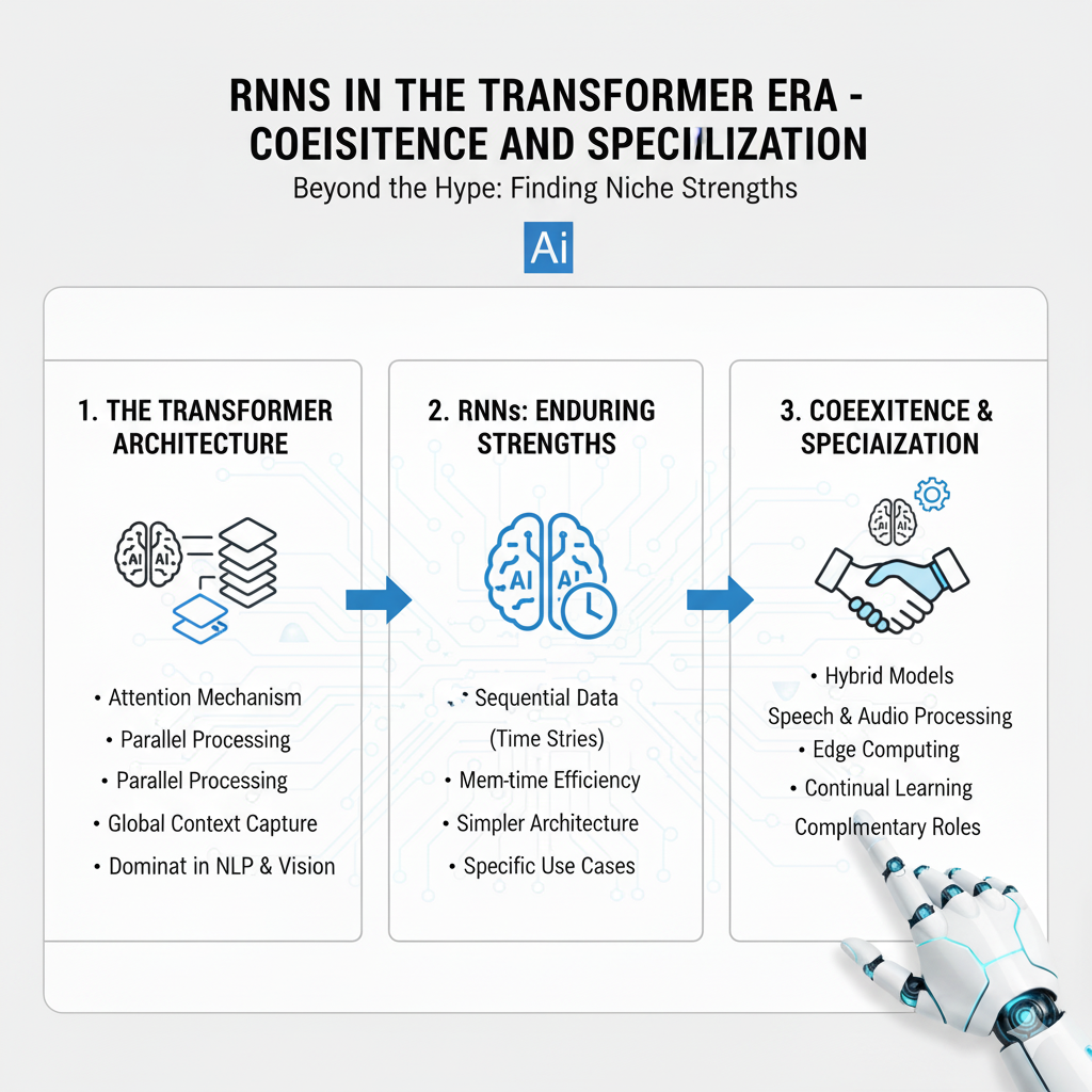
5.1 When to Choose RNNs in 2025:

• Streaming Data & Real-time Applications: RNNs process data sequentially, making them ideal for real-time predictions where you cannot wait for the entire sequence (e.g., live captioning, real-time anomaly detection).
• Resource-Constrained Environments: RNNs, especially optimized variants, typically have lower computational and memory requirements than equivalent Transformers.
• Long Sequences with Local Dependencies: For sequences where local context is most important and global attention is overkill.
• Edge Computing and Mobile Deployment: Their sequential nature and smaller memory footprint make them suitable for on-device AI.

5.2 The Hybrid Future: RNN-Transformer Architectures

Many state-of-the-art systems in 2025 use hybrid approaches:

python

# Conceptual example of an RNN-Transformer hybrid
def create_rnn_transformer_hybrid(seq_length, vocab_size):
    inputs = layers.Input(shape=(seq_length,))
    
    # RNN for local feature extraction
    embedding = layers.Embedding(vocab_size, 128)(inputs)
    rnn_features = layers.Bidirectional(layers.LSTM(64, return_sequences=True))(embedding)
    
    # Transformer for global context
    attention_output = layers.MultiHeadAttention(
        num_heads=4, key_dim=64)(rnn_features, rnn_features)
    
    # Combine both representations
    combined = layers.Concatenate()([rnn_features, attention_output])
    
    # Global pooling and classification
    pooled = layers.GlobalAveragePooling1D()(combined)
    outputs = layers.Dense(1, activation='sigmoid')(pooled)
    
    model = models.Model(inputs, outputs)
    return model

Part 6: Advanced Applications and Future Frontiers

RNNs continue to power innovative applications across industries. Here are the cutting-edge use cases in 2025:

6.1 Time Series Forecasting with Modern RNNs

python

def create_multivariate_rnn_forecaster(timesteps, features):
    """Creates an RNN for multivariate time series forecasting."""
    model = models.Sequential([
        layers.LSTM(128, return_sequences=True, input_shape=(timesteps, features)),
        layers.Dropout(0.3),
        layers.LSTM(64, return_sequences=True),
        layers.Dropout(0.3),
        layers.LSTM(32),
        layers.Dropout(0.3),
        layers.Dense(64, activation='swish'),
        layers.Dense(1)  # Predict single value
    ])
    
    model.compile(optimizer='adamw', loss='mse', metrics=['mae'])
    return model

# Application: Stock price prediction, energy demand forecasting, weather prediction

6.2 Anomaly Detection in Sequential Data

RNNs excel at learning normal patterns in sequences, making them perfect for detecting deviations that indicate fraud, system failures, or cybersecurity threats.

python

def create_lstm_autoencoder(seq_length, feature_dim):
    """LSTM Autoencoder for anomaly detection."""
    # Encoder
    inputs = layers.Input(shape=(seq_length, feature_dim))
    encoded = layers.LSTM(32, activation='swish', return_sequences=False)(inputs)
    encoded = layers.RepeatVector(seq_length)(encoded)
    
    # Decoder
    decoded = layers.LSTM(32, activation='swish', return_sequences=True)(encoded)
    decoded = layers.LSTM(feature_dim, activation='linear', return_sequences=True)(decoded)
    
    model = models.Model(inputs, decoded)
    model.compile(optimizer='adamw', loss='mse')
    return model

# Usage: High reconstruction error on test data indicates anomalies

6.3 Reinforcement Learning with RNNs

In deep reinforcement learning, RNNs serve as the “brain” for agents that need memory to operate in partially observable environments.

python

# Conceptual RNN-based Q-network for POMDPs
class RNNQNetwork(tf.keras.Model):
    def __init__(self, action_size, rnn_units=128):
        super(RNNQNetwork, self).__init__()
        self.lstm = layers.LSTM(rnn_units, return_sequences=True, return_state=True)
        self.dense1 = layers.Dense(64, activation='swish')
        self.dense2 = layers.Dense(32, activation='swish')
        self.q_values = layers.Dense(action_size, activation='linear')
        
    def call(self, inputs, initial_state=None, training=False):
        # inputs shape: (batch_size, seq_len, state_dim)
        lstm_out, state_h, state_c = self.lstm(inputs, initial_state=initial_state)
        # Use only the last output
        last_out = lstm_out[:, -1, :]
        x = self.dense1(last_out)
        x = self.dense2(x)
        q_values = self.q_values(x)
        return q_values, [state_h, state_c]

Part 7: The 2025 RNN Ecosystem – Emerging Trends and Production Realities

As we look toward the future of sequence modeling, several key trends and practical considerations are shaping how recurrent architectures are developed, deployed, and maintained in production environments. Understanding these evolving aspects is crucial for anyone working with temporal data in 2025.

7.1 Efficient Sequence Modeling: The Return of Linear Recurrence

A significant development in the sequence modeling space has been the resurgence of linear recurrence mechanisms that offer compelling alternatives to traditional gated architectures. Methods like S4 (Structured State Space) and Hyena have demonstrated that carefully designed linear recurrence can compete with, and sometimes surpass, both traditional recurrent models and attention-based approaches on long-range reasoning tasks.

These approaches leverage mathematical structures like state space models and convolutional representations to achieve parallel training while maintaining efficient sequential inference. The key insight is that many sequence modeling tasks don’t require the full expressive power of nonlinear gating at every step.

python

# Conceptual implementation of a simplified linear recurrent unit
class LinearRecurrentUnit(tf.keras.layers.Layer):
    def __init__(self, units, **kwargs):
        super(LinearRecurrentUnit, self).__init__(**kwargs)
        self.units = units
        
    def build(self, input_shape):
        # Learnable recurrence parameters
        self.A = self.add_weight(shape=(self.units, self.units),
                                initializer='orthogonal',
                                trainable=True)
        self.B = self.add_weight(shape=(input_shape[-1], self.units),
                                initializer='random_normal',
                                trainable=True)
        self.C = self.add_weight(shape=(self.units, self.units),
                                initializer='random_normal', 
                                trainable=True)
        
    def call(self, inputs):
        batch_size, seq_len, input_dim = tf.shape(inputs)[0], tf.shape(inputs)[1], tf.shape(inputs)[2]
        
        # Initialize hidden state
        h = tf.zeros((batch_size, self.units))
        outputs = []
        
        for t in range(seq_len):
            # Linear recurrence: h_t = A * h_{t-1} + B * x_t
            h = tf.matmul(h, self.A) + tf.matmul(inputs[:, t, :], self.B)
            # Output transformation
            output = tf.matmul(h, self.C)
            outputs.append(output)
            
        return tf.stack(outputs, axis=1)

The advantage of such approaches lies in their theoretical properties: better gradient flow, efficient long-range dependencies, and the potential for parallelized training through clever mathematical parameterizations.

7.2 Continuous-time Sequence Modeling

Traditional recurrent architectures operate on discrete time steps, which can be limiting for irregularly sampled time series or events that occur in continuous time. Recent advances in neural differential equations and continuous-time recurrent models provide a more natural framework for these scenarios.

python

# Conceptual continuous-time RNN using neural ODEs
class ContinuousTimeRNN(tf.keras.layers.Layer):
    def __init__(self, units, **kwargs):
        super(ContinuousTimeRNN, self).__init__(**kwargs)
        self.units = units
        
    def build(self, input_shape):
        # Parameters for the continuous dynamics
        self.W_h = self.add_weight(shape=(self.units, self.units))
        self.W_x = self.add_weight(shape=(input_shape[-1], self.units))
        self.bias = self.add_weight(shape=(self.units,))
        
    def ode_func(self, t, h, inputs):
        """Define the continuous dynamics: dh/dt = f(h, x)"""
        # Interpolate inputs at time t for continuous input handling
        x_t = self.interpolate_inputs(t, inputs)
        return tf.nn.tanh(tf.matmul(h, self.W_h) + tf.matmul(x_t, self.W_x) + self.bias)
    
    def call(self, inputs, times):
        # Solve the ODE: h(t) = h0 + ∫ f(h, x) dt from t0 to t1
        from diffeqpy import ode  # Using a differential equation solver
        
        h0 = tf.zeros((tf.shape(inputs)[0], self.units))
        solution = ode.solve(self.ode_func, h0, times, inputs)
        return solution

This approach is particularly valuable in domains like healthcare (modeling patient vitals), finance (irregular trades), and physics (sensor data), where measurements don’t arrive at regular intervals.

7.3 Memory-Augmented Architectures and External Memory

While traditional recurrent models maintain internal hidden states as their memory, there’s growing interest in architectures with explicit, external memory banks. These approaches, inspired by Neural Turing Machines and Differentiable Neural Computers, separate computation from memory storage.

python

class MemoryAugmentedRNN(tf.keras.layers.Layer):
    def __init__(self, units, memory_size, memory_dim, **kwargs):
        super(MemoryAugmentedRNN, self).__init__(**kwargs)
        self.units = units
        self.memory_size = memory_size
        self.memory_dim = memory_dim
        
    def build(self, input_shape):
        # Core RNN unit
        self.rnn_cell = tf.keras.layers.LSTMCell(self.units)
        
        # Memory mechanisms
        self.key_proj = tf.keras.layers.Dense(self.memory_dim)
        self.value_proj = tf.keras.layers.Dense(self.memory_dim)
        
    def call(self, inputs, training=None):
        batch_size = tf.shape(inputs)[0]
        seq_len = tf.shape(inputs)[1]
        
        # Initialize memory matrix
        memory = tf.zeros((batch_size, self.memory_size, self.memory_dim))
        
        # Initialize RNN state
        state = [tf.zeros((batch_size, self.units)), tf.zeros((batch_size, self.units))]
        
        outputs = []
        for t in range(seq_len):
            # Read from memory using content-based addressing
            read_weights = self.compute_read_weights(state[0], memory)
            read_vector = tf.reduce_sum(read_weights * memory, axis=1)
            
            # Combine current input with memory read
            combined_input = tf.concat([inputs[:, t, :], read_vector], axis=-1)
            
            # RNN step
            output, state = self.rnn_cell(combined_input, state, training=training)
            
            # Write to memory
            memory = self.memory_write(state[0], memory, read_weights)
            
            outputs.append(output)
            
        return tf.stack(outputs, axis=1)
    
    def compute_read_weights(self, query, memory):
        """Content-based addressing using cosine similarity"""
        query_expanded = tf.expand_dims(self.key_proj(query), 1)
        similarities = tf.reduce_sum(query_expanded * memory, axis=-1)
        return tf.nn.softmax(similarities, axis=-1)
    
    def memory_write(self, controller_state, memory, read_weights):
        """Update memory based on controller state and read location"""
        # Simplified write operation - in practice would be more sophisticated
        write_vector = self.value_proj(controller_state)
        write_vector_expanded = tf.expand_dims(write_vector, 1)
        
        # Erase and add mechanism
        erase_gate = tf.nn.sigmoid(self.erase_proj(controller_state))
        add_gate = tf.nn.sigmoid(self.add_proj(controller_state))
        
        memory = memory * (1 - read_weights * erase_gate)
        memory = memory + read_weights * add_gate * write_vector_expanded
        
        return memory

These architectures show particular promise for tasks requiring complex reasoning, multi-step planning, and knowledge-intensive applications where explicit memory management is beneficial.

7.4 Production Considerations and Model Optimization

Deploying recurrent models in production environments requires careful consideration of several practical factors:

Quantization and Compression:

python

def optimize_rnn_for_deployment(model_path, output_path):
    """Optimize an RNN model for production deployment."""
    # Load the trained model
    model = tf.keras.models.load_model(model_path)
    
    # Create a converter with optimization
    converter = tf.lite.TFLiteConverter.from_keras_model(model)
    
    # Set optimization strategies
    converter.optimizations = [tf.lite.Optimize.DEFAULT]
    
    # For RNNs, we might want dynamic range quantization
    converter.representative_dataset = representative_dataset_gen
    
    # Optional: Full integer quantization for maximum performance
    converter.target_spec.supported_ops = [tf.lite.OpsSet.TFLITE_BUILTINS_INT8]
    converter.inference_input_type = tf.int8
    converter.inference_output_type = tf.int8
    
    # Convert and save
    tflite_model = converter.convert()
    
    with open(output_path, 'wb') as f:
        f.write(tflite_model)
    
    print(f"Optimized model saved to {output_path}")

def representative_dataset_gen():
    """Generate representative data for quantization calibration."""
    for _ in range(100):
        # Yield sample inputs that represent typical inference data
        yield [np.random.randint(0, 10000, (1, 500)).astype(np.int32)]

Streaming Inference and State Management:
For real-time applications, maintaining state across multiple inference calls is crucial:

python

class StreamingRNNPredictor:
    def __init__(self, model_path, sequence_length=500):
        self.model = tf.keras.models.load_model(model_path)
        self.sequence_length = sequence_length
        self.reset_state()
        
    def reset_state(self):
        """Reset the internal state for new sequences."""
        # Get initial state from the model
        self.state = [tf.zeros((1, layer.units)) for layer in self.model.layers 
                     if hasattr(layer, 'states')]
        self.buffer = []
        
    def predict_streaming(self, new_input):
        """Make predictions on streaming data."""
        self.buffer.append(new_input)
        
        # Maintain fixed sequence length
        if len(self.buffer) > self.sequence_length:
            self.buffer.pop(0)
            
        # Prepare input sequence
        if len(self.buffer) < self.sequence_length:
            # Pad if necessary
            padded_input = self.buffer + [0] * (self.sequence_length - len(self.buffer))
        else:
            padded_input = self.buffer
            
        input_tensor = tf.convert_to_tensor([padded_input])
        
        # Predict with stateful execution
        prediction, new_state = self.model

Conclusion: The Enduring Relevance of RNNs in 2025

The narrative that Transformers have completely replaced RNNs is a misconception. In 2025, RNNs remain vital, powerful tools in the deep learning arsenal. Their strengths—computational efficiency, suitability for streaming data, and excellent performance on many sequence tasks—ensure their continued relevance.

Mastering RNNs in the current landscape means:

1. Understanding the fundamentals of recurrence, LSTMs, and GRUs.
2. Implementing modern best practices like bidirectional processing, attention mechanisms, and proper regularization.
3. Knowing when to choose RNNs over Transformers based on the specific problem constraints.
4. Leveraging hybrid approaches that combine the strengths of multiple architectures.

The future of sequence modeling is not about one architecture winning, but about having the wisdom to select and combine the right tools for each challenge. By mastering RNNs, you equip yourself with a timeless, powerful technology for turning the flow of time into actionable intelligence.