Master CNN in 2025: Transform Images into Intelligence with Deep Learning

Master CNN in 2025 with our complete guide. Learn convolutional neural networks from basics to advanced architectures like EfficientNet, Transformers, and 3D CNNs. Includes Python code, transfer learning, and deployment strategies for real-world computer vision applications.

Introduction: The Indispensable Engine of Visual AI

In the data-rich landscape of 2025, visual information is no longer just a medium; it’s the lifeblood of innovation. From medical diagnostics that analyze 3D organ scans to autonomous vehicles navigating complex urban environments, the ability to extract meaning from pixels is a foundational capability. At the heart of this visual intelligence revolution lies a specific and powerful class of deep learning models: the Convolutional Neural Network, or CNN.

A CNN is a specialized neural network architecture designed to process data with a grid-like topology, most notably images. Its biological inspiration comes from the animal visual cortex, where small, overlapping regions of the visual field are processed by individual neurons. This architectural design allows CNNs to automatically and adaptively learn spatial hierarchies of features, from low-level edges and textures to high-level object parts and complex scenes.

Mastering CNNs in 2025 is not just about understanding their core mechanics; it’s about leveraging their evolved capabilities to solve real-world problems with unprecedented accuracy and efficiency. This guide will take you from the fundamental principles that make CNNs work to the advanced architectures and techniques defining the state-of-the-art, empowering you to transform raw pixels into actionable intelligence.

Part 1: The Foundational Blocks – Deconstructing the CNN Engine

To master CNNs, one must first understand the purpose and function of their core components. These layers work in concert to break down an image into a meaningful representation.

1.1 The Convolutional Layer: The Feature Detector

This is the layer that gives the CNN its name. Its primary function is to detect features—such as edges, corners, and color contrasts—regardless of their position in the image.

• How it Works: The layer uses a set of learnable filters (or kernels). Each filter is a small window (e.g., 3×3 or 5×5 pixels) that slides, or “convolves,” across the width and height of the input image. At every location, it performs a dot product between the filter values and the underlying pixel values of the input. This process creates a 2D activation map called a feature map.
  • Stride: The number of pixels the filter moves each time. A stride of 1 moves the filter one pixel at a time; a stride of 2 moves it two pixels, producing a smaller output.
  • Padding: To prevent the feature map from shrinking too quickly, we often pad the input with zeros around the border. “Same” padding ensures the output has the same spatial dimensions as the input.
• The “Learning” Part: Initially, the filter values are random. During training, through backpropagation, the network learns the optimal values for these filters. One filter might learn to activate in the presence of a vertical edge, while another might learn to detect a specific shade of blue.

1.2 The Pooling Layer: The Information Concentrator

Pooling layers are used to progressively reduce the spatial size of the representation, which reduces the computational load, memory usage, and number of parameters. This also helps to control overfitting by providing an abstracted form of the representation.

• Max Pooling: The most common type. It partitions the feature map into rectangles and outputs the maximum value for each region. For example, a 2×2 max pool with a stride of 2 will reduce the feature map size by 75%. It retains the most salient features.
• Average Pooling: Outputs the average value of the region. It is less common but can be used in the final layers of some architectures.

Pooling introduces translation invariance, meaning the network becomes less sensitive to the exact position of a feature, focusing more on its presence.

1.3 The Fully Connected Layer: The Classifier

After several rounds of convolution and pooling, the high-level reasoning in the network is done via fully connected (FC) layers. These layers are identical to those in a standard Multilayer Perceptron (MLP). The 2D feature maps are flattened into a 1D vector and fed into the FC layers, which combine these features to perform the final classification (e.g., “this is a cat”) or regression.

1.4 Activation Functions: Introducing Non-Linearity

Without non-linearity, a deep network would be equivalent to a single linear transformation. Activation functions are applied element-wise after convolutional and fully connected layers to allow the network to learn complex, non-linear patterns.

• ReLU (Rectified Linear Unit): The default choice for years, f(x) = max(0, x). It’s computationally efficient and mitigates the vanishing gradient problem.
• Leaky ReLU & Parametric ReLU (PReLU): Advanced variants that allow a small, non-zero gradient when the unit is not active, preventing “dying ReLU” problems.
• Swish / SiLU: A newer, self-gated activation function (f(x) = x * sigmoid(x)) that has been shown to often outperform ReLU in very deep networks and is a default in many 2025 models.

Part 2: A Practical Walkthrough – Building a CNN from Scratch in 2025

Let’s solidify these concepts by building a modern CNN for a classic problem: image classification on the CIFAR-10 dataset, using TensorFlow/Keras with 2025 best practices.

python

import tensorflow as tf
from tensorflow.keras import layers, models, regularizers
import matplotlib.pyplot as plt

# Load and preprocess the CIFAR-10 dataset
(x_train, y_train), (x_test, y_test) = tf.keras.datasets.cifar10.load_data()

# Normalize pixel values to [0, 1] and convert labels to categorical
x_train, x_test = x_train / 255.0, x_test / 255.0
y_train = tf.keras.utils.to_categorical(y_train, 10)
y_test = tf.keras.utils.to_categorical(y_test, 10)

print(f"Training data shape: {x_train.shape}") # (50000, 32, 32, 3)
print(f"Test data shape: {x_test.shape}")     # (10000, 32, 32, 3)

def create_modern_cnn(input_shape=(32, 32, 3), num_classes=10):
    """Creates a CNN with modern architectural practices."""
    model = models.Sequential()

    # First Convolutional Block: Feature Extraction Foundation
    model.add(layers.Conv2D(32, (3, 3), padding='same', input_shape=input_shape))
    model.add(layers.BatchNormalization())  # Standard in 2025: Batchnorm before activation
    model.add(layers.Activation('swish'))   # Modern activation function
    model.add(layers.Conv2D(32, (3, 3), padding='same'))
    model.add(layers.BatchNormalization())
    model.add(layers.Activation('swish'))
    model.add(layers.MaxPooling2D((2, 2)))
    model.add(layers.Dropout(0.25))  # Dropout for regularization

    # Second Convolutional Block: Learning More Complex Features
    model.add(layers.Conv2D(64, (3, 3), padding='same'))
    model.add(layers.BatchNormalization())
    model.add(layers.Activation('swish'))
    model.add(layers.Conv2D(64, (3, 3), padding='same'))
    model.add(layers.BatchNormalization())
    model.add(layers.Activation('swish'))
    model.add(layers.MaxPooling2D((2, 2)))
    model.add(layers.Dropout(0.25))

    # Third Convolutional Block: High-Level Abstraction
    model.add(layers.Conv2D(128, (3, 3), padding='same'))
    model.add(layers.BatchNormalization())
    model.add(layers.Activation('swish'))
    model.add(layers.GlobalAveragePooling2D()) # Modern alternative to Flatten + Dense: reduces parameters

    # Final Classification Block
    model.add(layers.Dense(128, activation='swish', kernel_regularizer=regularizers.l2(1e-4)))
    model.add(layers.Dropout(0.5))
    model.add(layers.Dense(num_classes, activation='softmax'))

    return model

# Create and compile the model
model = create_modern_cnn()

model.compile(optimizer='adamw',  # AdamW is Adam with decoupled weight decay
              loss='categorical_crossentropy',
              metrics=['accuracy'])

# Display the architecture
model.summary()

# Define callbacks for a robust training process
callbacks = [
    tf.keras.callbacks.ReduceLROnPlateau(monitor='val_loss', factor=0.5, patience=5, min_lr=1e-7),
    tf.keras.callbacks.EarlyStopping(monitor='val_loss', patience=15, restore_best_weights=True),
]

# Train the model
history = model.fit(x_train, y_train,
                    batch_size=128,
                    epochs=100,
                    validation_data=(x_test, y_test),
                    callbacks=callbacks,
                    verbose=1)

# Evaluate the final model
test_loss, test_accuracy = model.evaluate(x_test, y_test, verbose=0)
print(f"\nFinal Test Accuracy: {test_accuracy:.4f}")

# Plot training history
plt.figure(figsize=(12, 4))
plt.subplot(1, 2, 1)
plt.plot(history.history['accuracy'], label='Training Accuracy')
plt.plot(history.history['val_accuracy'], label='Validation Accuracy')
plt.title('Model Accuracy')
plt.legend()
plt.subplot(1, 2, 2)
plt.plot(history.history['loss'], label='Training Loss')
plt.plot(history.history['val_loss'], label='Validation Loss')
plt.title('Model Loss')
plt.legend()
plt.show()

Key 2025 Takeaways from this Code:

• Batch Normalization: Used after almost every convolution to stabilize and accelerate training.
• Swish Activation: A modern, often superior alternative to ReLU.
• Global Average Pooling (GAP): Replaces the traditional “Flatten + Dense” layer, drastically reducing parameters and combating overfitting.
• AdamW Optimizer: The standard optimizer with improved weight decay handling.
• Structured Regularization: A combination of Dropout and L2 regularization to prevent overfitting.
• Sophisticated Callbacks: ReduceLROnPlateau and EarlyStopping automate learning rate adjustment and prevent overtraining.

Part 3: The Evolution of Power – Key CNN Architectures You Must Know

The history of CNNs is marked by a few landmark architectures that pushed the boundaries of what was possible. Understanding this evolution is key to mastering their application.

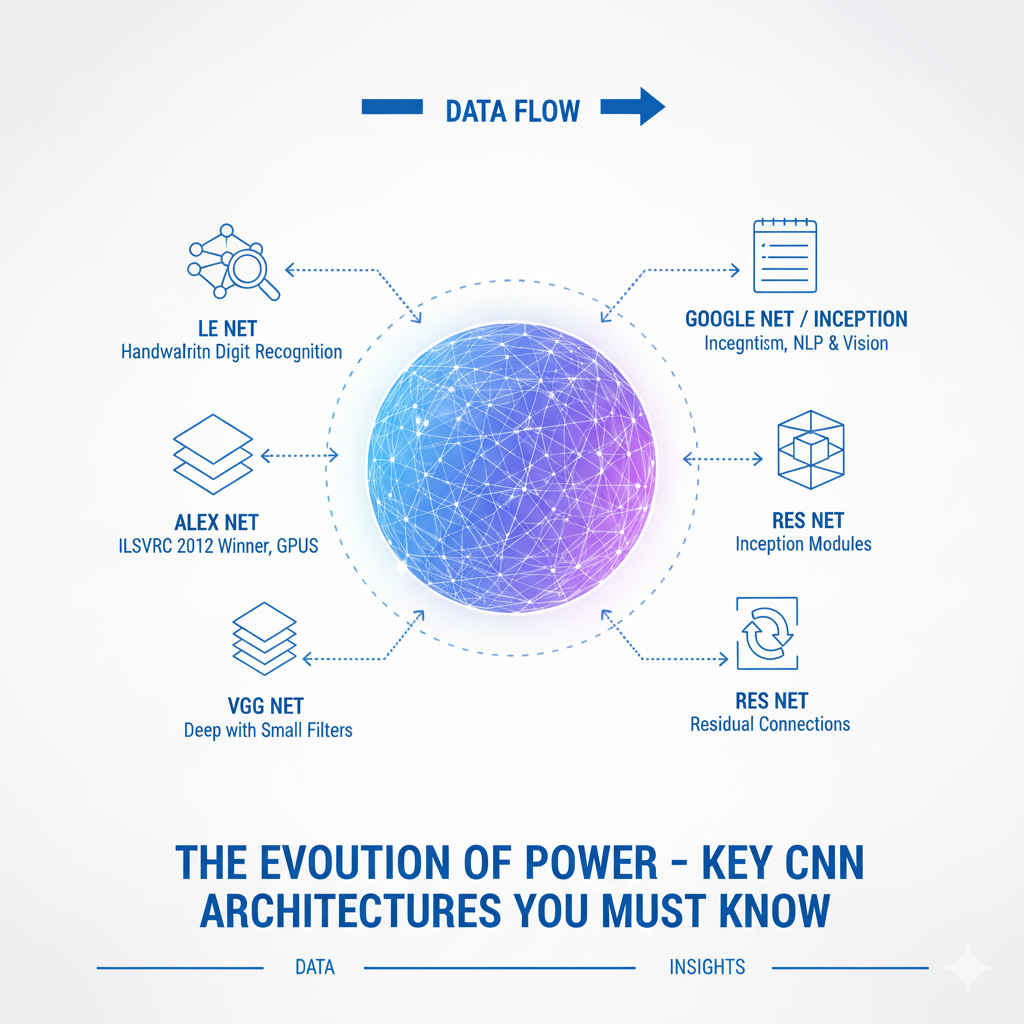
3.1 The Pioneers: LeNet-5, AlexNet

• LeNet-5 (1998): The pioneering architecture by Yann LeCun for handwritten digit recognition. It established the classic pattern: Convolution -> Pooling -> Convolution -> Pooling -> Fully Connected -> Output.
• AlexNet (2012): The model that sparked the deep learning revolution. It won the ImageNet competition by a large margin, proving the power of deep CNNs with GPUs. It used ReLU, Dropout, and data augmentation.

3.2 The Depth Revolution: VGGNet, Inception, ResNet

• VGGNet (2014): Demonstrated that depth is a critical component for performance. Its simple, modular architecture of 3×3 convolutions stacked to a depth of 16-19 layers became a standard reference.
• Inception (GoogLeNet, 2014): Introduced the “Inception module,” which performs multiple convolutions (e.g., 1×1, 3×3, 5×5) and pooling in parallel and concatenates the results. This allows the network to choose the best filter size for each region, making it computationally efficient.
• ResNet (2015): A groundbreaking architecture that solved the “vanishing gradient” problem in very deep networks (100+ layers). It introduced skip connections (or residual connections), which allow the gradient to flow directly through the network. This made it possible to train extremely deep models, and ResNet variants remain a top choice in 2025.

3.3 The 2025 Standard-Bearers: EfficientNet, ConvNeXt

• EfficientNet (2019): A family of models that uses a compound scaling method to uniformly scale up network depth, width, and resolution. It achieves state-of-the-art accuracy with an order of magnitude fewer parameters and FLOPS, making it ideal for production environments in 2025.
• ConvNeXt (2022): A modern re-imagining of the classic ResNet design, incorporating design principles from Vision Transformers (ViTs). It uses larger kernel sizes (7×7), inverted bottlenecks, and modern activation and normalization techniques, often outperforming both ResNet and ViTs on standard benchmarks.

Part 4: Beyond Classification – The Versatile Applications of CNNs in 2025

The utility of CNNs extends far beyond telling cats from dogs. They are the backbone of numerous advanced computer vision tasks.

4.1 Object Detection: Not Just “What” but “Where”

Object detection involves classifying objects and localizing them with bounding boxes. Modern detectors are built upon CNNs.

• Two-Stage Detectors: Models like Faster R-CNN use a CNN (a Region Proposal Network) to first propose regions of interest and then a second network to classify and refine those regions. High accuracy, slower speed.
• Single-Stage Detectors: Models like YOLO (You Only Look Once) and SSD (Single Shot MultiBox Detector) treat detection as a single regression problem, directly predicting bounding boxes and class probabilities from the image in one pass. Extremely fast, ideal for real-time applications like video analysis and autonomous driving.

4.2 Semantic Segmentation: A Label for Every Pixel

This task requires assigning a class label to every single pixel in the image, effectively understanding the image at a pixel level.

• U-Net: A seminal architecture with an encoder-decoder structure and “skip connections” that combine high-resolution features from the encoder with the upsampled decoder features. It’s the gold standard for medical image segmentation (e.g., identifying tumors in MRI scans).
• DeepLab: Uses atrous (dilated) convolutions to capture multi-scale contextual information without losing resolution, and Atrous Spatial Pyramid Pooling (ASPP) to segment objects at multiple scales effectively.

4.3 Transfer Learning: The Practitioner’s Superpower

In 2025, it is rare to train a large CNN from scratch on a small dataset. The standard practice is Transfer Learning.

• Concept: Take a CNN pre-trained on a massive dataset like ImageNet (which contains 1.2 million images across 1000 classes). This model has already learned to recognize a vast dictionary of general features.
• Process:
  1. Remove the final classification layer of the pre-trained model.
  2. Freeze the weights of the earlier (feature-extraction) layers.
  3. Add new, randomly initialized layers on top tailored to your specific task (e.g., a new classifier for your 10 classes).
  4. Train only the new layers on your dataset.
• Fine-Tuning: For even better performance, you can later “unfreeze” some of the deeper layers of the base model and train them with a very low learning rate, allowing the features to specialize for your domain.

python

# Example of Transfer Learning with EfficientNet in 2025
def create_model_using_transfer_learning(num_classes=10):
    # Load a pre-trained EfficientNet backbone, excluding its top classifier
    base_model = tf.keras.applications.EfficientNetB0(
        include_top=False,
        weights='imagenet',
        input_shape=(32, 32, 3) # Note: EfficientNet expects larger images, this is for demo
    )
    base_model.trainable = False  # Freeze the base model

    # Create a new model on top
    inputs = tf.keras.Input(shape=(32, 32, 3))
    # We use the base model as a feature extractor
    x = base_model(inputs, training=False)
    x = layers.GlobalAveragePooling2D()(x)
    # Add a new classifier
    outputs = layers.Dense(num_classes, activation='softmax')(x)

    model = tf.keras.Model(inputs, outputs)
    return model

transfer_model = create_model_using_transfer_learning()
transfer_model.compile(optimizer='adam', loss='categorical_crossentropy', metrics=['accuracy'])

Part 5: Mastering the Craft – Advanced Techniques and Best Practices for 2025

Building a high-performing CNN requires more than just stacking layers. It involves a deep understanding of the training process and advanced regularization techniques.

5.1 Combatting Overfitting: A Multi-Front Battle

Overfitting is the enemy of generalization. A 2025 practitioner’s toolkit is full of weapons to fight it.

• Data Augmentation: Artificially expanding your training dataset by creating modified versions of your images. This teaches the model to be invariant to changes in rotation, scale, brightness, etc. In 2025, this is done on-the-fly during training.python# Real-time data augmentation in Keras from tensorflow.keras.preprocessing.image import ImageDataGenerator datagen = ImageDataGenerator( rotation_range=20, width_shift_range=0.2, height_shift_range=0.2, horizontal_flip=True, zoom_range=0.2, fill_mode=’nearest’ ) # Use `datagen.flow(x_train, y_train, batch_size=32)` during model.fit
• Advanced Regularization:
  • Dropout: As seen in our model, it randomly “drops out” a percentage of neurons during training, preventing complex co-adaptations.
  • Weight Decay (L2 Regularization): Adds a penalty to the loss function for large weights, encouraging a simpler model.
  • Stochastic Depth: Randomly drops entire layers during training, a technique popularized in ResNet variants.
  • Label Smoothing: Replaces one-hot encoded labels with a small mixture of the other classes, preventing the model from becoming overconfident.

5.2 Optimization and Training Dynamics

• Optimizers: Adam/AdamW is the default. For ultimate performance, sometimes SGD with Nesterov momentum and a careful learning rate schedule can yield better results, though it requires more tuning.
• Learning Rate Schedulers: Critical for convergence. ReduceLROnPlateau is a good default. CosineAnnealing is a powerful modern scheduler that reduces the learning rate in a cosine pattern, often leading to better generalization.

5.3 Interpretability: Opening the Black Box

In 2025, understanding why a CNN made a decision is crucial for trust and debugging, especially in fields like healthcare.

• Grad-CAM (Gradient-weighted Class Activation Mapping): A technique that produces a heatmap highlighting the important regions in the image for a particular prediction. It answers the question: “Where did the model look to decide this was a ‘cat’?”
• SHAP (SHapley Additive exPlanations) and LIME: Model-agnostic methods that can approximate the contribution of each pixel to the final prediction.

Part 6: The 2025 CNN Ecosystem – Emerging Trends and Future Frontiers

As we move deeper into the decade, the CNN landscape is not static. While foundational principles remain, new architectural innovations, training paradigms, and application domains are pushing the boundaries of what’s possible. Mastering CNNs in 2025 requires an understanding of these emerging frontiers.

6.1 The CNN vs. Transformer Synthesis: The Best of Both Worlds

The rise of Vision Transformers (ViTs) created a significant debate: are Transformers destined to replace CNNs for computer vision? The answer in 2025 is increasingly nuanced, leading to powerful hybrid architectures.

• The Strengths of ViTs: Transformers excel at capturing global context and long-range dependencies through their self-attention mechanism. They can understand how every part of an image relates to every other part, which is particularly valuable for complex scenes.
• The Enduring Strengths of CNNs: CNNs maintain superior inductive biases for images—translation equivariance and locality—meaning they require less data to learn effective representations and are computationally more efficient for high-resolution images.

The Hybrid Future: Convolutional Transformers
The most exciting development is the synthesis of these approaches. Models like Convolutional Vision Transformers (CvT) and CoAtNets integrate convolutional operations into the Transformer architecture.

• How they work: These models typically use a CNN-like stem (initial layers) to process the image into patch embeddings, leveraging the spatial efficiency of convolutions. They then apply Transformer blocks that may use convolutional projections instead of standard linear projections for the Query, Key, and Value matrices. This combines the local feature extraction power of CNNs with the global reasoning capability of Transformers.

python

# Conceptual example of a hybrid Conv-Transformer block
class ConvTransformerBlock(tf.keras.layers.Layer):
    def __init__(self, embed_dim, num_heads, ff_dim, rate=0.1):
        super(ConvTransformerBlock, self).__init__()
        # Multi-Head Attention with convolutional projections
        self.att = layers.MultiHeadAttention(num_heads=num_heads, key_dim=embed_dim)
        self.conv_q = layers.Conv2D(embed_dim, 1)  # 1x1 convolution for query projection
        self.conv_k = layers.Conv2D(embed_dim, 1)  # 1x1 convolution for key projection
        self.conv_v = layers.Conv2D(embed_dim, 1)  # 1x1 convolution for value projection
        
        # Feed-forward network
        self.ffn = tf.keras.Sequential([
            layers.Dense(ff_dim, activation="swish"),
            layers.Dense(embed_dim),
        ])
        self.layernorm1 = layers.LayerNormalization(epsilon=1e-6)
        self.layernorm2 = layers.LayerNormalization(epsilon=1e-6)
        self.dropout1 = layers.Dropout(rate)
        self.dropout2 = layers.Dropout(rate)

    def call(self, inputs, training):
        # inputs shape: (batch_size, height, width, channels)
        batch_size, h, w, c = inputs.shape
        
        # Convolutional projections for attention
        q = self.conv_q(inputs)  # Shape remains (batch_size, h, w, c)
        k = self.conv_k(inputs)
        v = self.conv_v(inputs)
        
        # Reshape for attention: (batch_size, h*w, c)
        q_flat = tf.reshape(q, [batch_size, h * w, c])
        k_flat = tf.reshape(k, [batch_size, h * w, c])
        v_flat = tf.reshape(v, [batch_size, h * w, c])
        
        # Multi-head attention
        attn_output = self.att(q_flat, k_flat, v_flat, training=training)
        attn_output = self.dropout1(attn_output, training=training)
        
        # Reshape back and add residual
        attn_output = tf.reshape(attn_output, [batch_size, h, w, c])
        out1 = self.layernorm1(inputs + attn_output)
        
        # Feed-forward network
        ffn_output = self.ffn(out1)
        ffn_output = self.dropout2(ffn_output, training=training)
        out2 = self.layernorm2(out1 + ffn_output)
        
        return out2

6.2 Attention Mechanisms in CNNs: Learning What to Focus On

While Transformers brought attention to the forefront, attention mechanisms have been successfully integrated into pure CNN architectures, creating more efficient and powerful models.

• Squeeze-and-Excitation (SE) Networks: Introduces a lightweight gating mechanism that models channel-wise relationships. It “squeezes” global spatial information into a channel descriptor, then “excites” (recalibrates) channel-wise feature responses by modeling dependencies between channels.
• Convolutional Block Attention Module (CBAM): A sequential attention module that applies both channel attention and spatial attention in sequence, telling the network not only “what” to focus on but also “where.”

python

# Implementation of a simplified Squeeze-and-Excitation block
class SEBlock(tf.keras.layers.Layer):
    def __init__(self, ratio=16):
        super(SEBlock, self).__init__()
        self.ratio = ratio
        self.gap = layers.GlobalAveragePooling2D()
        self.dense1 = layers.Dense(units=0, use_bias=False)  # Will be set in build()
        self.dense2 = layers.Dense(units=0, use_bias=False)  # Will be set in build()
        self.relu = layers.ReLU()
        self.sigmoid = layers.Activation('sigmoid')

    def build(self, input_shape):
        filters = input_shape[-1]
        self.reduction_units = max(1, filters // self.ratio)
        self.dense1.units = self.reduction_units
        self.dense2.units = filters
        super(SEBlock, self).build(input_shape)

    def call(self, inputs):
        # Squeeze: Global Average Pooling
        se = self.gap(inputs)  # Shape: (batch_size, channels)
        
        # Excitation: Two fully connected layers
        se = self.dense1(se)
        se = self.relu(se)
        se = self.dense2(se)
        se = self.sigmoid(se)  # Shape: (batch_size, channels)
        
        # Scale: Multiply original input with attention weights
        se = tf.reshape(se, [-1, 1, 1, tf.shape(se)[-1]])  # Reshape for broadcasting
        return inputs * se

# Using SE Block in a CNN
def create_se_cnn():
    model = models.Sequential([
        layers.Conv2D(32, 3, padding='same', input_shape=(32, 32, 3)),
        layers.BatchNormalization(),
        layers.Activation('swish'),
        SEBlock(ratio=16),  # Add attention here
        layers.MaxPooling2D(2),
        # ... more layers
    ])
    return model

6.3 Neural Architecture Search (NAS) and Automated CNN Design

In 2025, the design of optimal CNN architectures is increasingly being automated through Neural Architecture Search (NAS). Instead of human engineers designing architectures through trial and error, NAS algorithms automatically discover high-performing architectures for specific tasks and constraints.

• How NAS Works: NAS typically involves three components:
  1. Search Space: The set of possible operations (convolution types, kernel sizes, connections) and how they can be connected.
  2. Search Strategy: The method for exploring the search space (reinforcement learning, evolutionary algorithms, gradient-based methods).
  3. Performance Estimation: How to quickly evaluate candidate architectures (weight sharing, proxy tasks, lower fidelity training).
• Popular NAS-derived Architectures:
  • EfficientNet: The result of compound scaling discovered through NAS.
  • RegNet: A design space that is both simple and rich, leading to models that outperform many hand-designed and NAS-discovered architectures.
  • MobileNetV3: Optimized for mobile devices using NAS and NetAdapt algorithms.

python

# Example of using an AutoML approach with KerasTuner
!pip install keras-tuner -q

import keras_tuner as kt

def build_model(hp):
    model = tf.keras.Sequential()
    
    # Tune the number of convolutional blocks
    for i in range(hp.Int('num_blocks', 2, 5)):
        # Tune the number of filters
        filters = hp.Choice(f'filters_{i}', values=[32, 64, 128, 256])
        model.add(layers.Conv2D(filters, 3, padding='same', activation='swish'))
        model.add(layers.BatchNormalization())
        if hp.Boolean(f'use_se_{i}'):  # Tune whether to use SE attention
            model.add(SEBlock())
        model.add(layers.MaxPooling2D(2))
        model.add(layers.Dropout(hp.Float(f'dropout_{i}', 0.1, 0.5, step=0.1)))
    
    model.add(layers.GlobalAveragePooling2D())
    model.add(layers.Dense(10, activation='softmax'))
    
    # Tune the learning rate
    learning_rate = hp.Float('lr', 1e-4, 1e-2, sampling='log')
    model.compile(optimizer=tf.keras.optimizers.Adam(learning_rate=learning_rate),
                  loss='categorical_crossentropy',
                  metrics=['accuracy'])
    return model

# Initialize the tuner
tuner = kt.BayesianOptimization(
    build_model,
    objective='val_accuracy',
    max_trials=20,
    executions_per_trial=1,
    directory='nas_dir',
    project_name='cnn_architecture_search'
)

# Run the search
tuner.search(x_train, y_train, 
             epochs=20, 
             validation_data=(x_test, y_test),
             callbacks=[tf.keras.callbacks.EarlyStopping('val_accuracy', patience=5)])

# Get the best model
best_model = tuner.get_best_models(num_models=1)[0]

6.4 3D CNNs and Video Understanding

While 2D CNNs excel at image analysis, the world is inherently three-dimensional and temporal. 3D CNNs extend the convolution operation to spatiotemporal data, making them essential for video analysis, medical imaging, and scientific data.

• 3D Convolutions: Instead of 2D filters that slide across width and height, 3D filters slide across width, height, and depth (time or spatial depth).
• Applications:
  • Video Action Recognition: Classifying human actions in video sequences.
  • Medical Image Analysis: Processing 3D MRI, CT scans for tumor detection and organ segmentation.
  • Autonomous Driving: Understanding temporal sequences of LiDAR or camera data.

python

# 3D CNN for video action recognition
def create_3d_cnn(input_shape=(16, 112, 112, 3), num_classes=10):  # (frames, height, width, channels)
    model = tf.keras.Sequential([
        # First 3D Convolutional Block
        layers.Conv3D(32, (3, 3, 3), activation='swish', padding='same', input_shape=input_shape),
        layers.BatchNormalization(),
        layers.MaxPooling3D((1, 2, 2)),  # Reduce spatial dimensions
        
        # Second 3D Convolutional Block  
        layers.Conv3D(64, (3, 3, 3), activation='swish', padding='same'),
        layers.BatchNormalization(),
        layers.MaxPooling3D((2, 2, 2)),  # Reduce both temporal and spatial dimensions
        
        # Third 3D Convolutional Block
        layers.Conv3D(128, (3, 3, 3), activation='swish', padding='same'),
        layers.BatchNormalization(),
        layers.MaxPooling3D((2, 2, 2)),
        
        # Global pooling and classification
        layers.GlobalAveragePooling3D(),
        layers.Dense(256, activation='swish'),
        layers.Dropout(0.5),
        layers.Dense(num_classes, activation='softmax')
    ])
    return model

# Note: 3D CNNs are computationally intensive and require significant memory

6.5 Edge AI and Efficient CNN Deployment

In 2025, the deployment of CNNs has moved beyond powerful servers to edge devices—mobile phones, IoT devices, embedded systems, and drones. This requires specialized optimization techniques.

• Model Quantization: Reducing the precision of weights and activations from 32-bit floating point to 16-bit, 8-bit integers, or even lower. This dramatically reduces model size and inference time with minimal accuracy loss.
• Model Pruning: Removing redundant weights or entire neurons that contribute little to the output, creating sparse models.
• Knowledge Distillation: Training a small, efficient “student” model to mimic the behavior of a large, accurate “teacher” model.
• Hardware-Aware Neural Architecture Search: Designing architectures specifically optimized for target hardware.

python

# Example of post-training quantization in TensorFlow Lite
def convert_to_tflite(model_path, save_path):
    # Load your trained model
    model = tf.keras.models.load_model(model_path)
    
    # Create a converter
    converter = tf.lite.TFLiteConverter.from_keras_model(model)
    
    # Set optimization options
    converter.optimizations = [tf.lite.Optimize.DEFAULT]
    
    # Optional: For full integer quantization
    # converter.representative_dataset = representative_dataset_gen
    # converter.target_spec.supported_ops = [tf.lite.OpsSet.TFLITE_BUILTINS_INT8]
    # converter.inference_input_type = tf.uint8
    # converter.inference_output_type = tf.uint8
    
    # Convert the model
    tflite_model = converter.convert()
    
    # Save the quantized model
    with open(save_path, 'wb') as f:
        f.write(tflite_model)
    
    print(f"Model converted and saved to {save_path}")
    print(f"Original model size: {os.path.getsize(model_path) / 1e6:.1f} MB")
    print(f"Quantized model size: {len(tflite_model) / 1e6:.1f} MB")

# Usage for mobile deployment
# convert_to_tflite('my_cnn_model.h5', 'my_cnn_quantized.tflite')

The Path Forward: Continuous Learning in the CNN Ecosystem

The CNN landscape in 2025 is dynamic and multifaceted. True mastery requires:

1. Staying Current with Research: Following developments in hybrid architectures, attention mechanisms, and optimization techniques.
2. Practical Experimentation: Implementing and testing new architectures on your specific domain problems.
3. Understanding Deployment Constraints: Considering model size, inference speed, and hardware requirements from the beginning of your projects.
4. Embracing Automation: Leveraging tools like NAS and AutoML to discover optimal architectures for your specific use cases.

The future of CNNs is not about replacement by newer architectures, but rather integration and specialization. By understanding these emerging trends, you position yourself at the forefront of visual AI, ready to leverage the right combination of techniques for any computer vision challenge in 2025 and beyond.

Conclusion: Your Path to CNN Mastery in the Visual AI Era

The Convolutional Neural Network has matured from an academic curiosity into the most reliable and versatile engine for visual understanding. Mastering it in 2025 means moving beyond theory to a practical, nuanced understanding of its components, its evolved architectures, and the ecosystem of techniques that surround it.

Your journey involves:

1. Solidifying the Fundamentals: Internalize the roles of convolution, pooling, and activation.
2. Embracing Modern Architectures: Leverage the power of ResNet, EfficientNet, and ConvNeXt through transfer learning.
3. Expanding Your Toolbox: Apply CNNs to detection, segmentation, and beyond.
4. Mastering the Craft: Use advanced regularization, optimization, and interpretability techniques to build robust, production-ready models.

The world is becoming increasingly visual. By mastering the CNN, you equip yourself with the fundamental tool to not just analyze this world, but to build the intelligent systems that will shape its future. The pixels are waiting; it’s time to transform them into intelligence.