Introduction: The Unseen Force Powering Modern AI
In the dazzling world of 2025’s artificial intelligence, where models generate photorealistic images, hold fluid conversations, and drive autonomous vehicles, a single, foundational algorithm operates silently in the background powering nearly every breakthrough. This algorithm is Backpropagation.
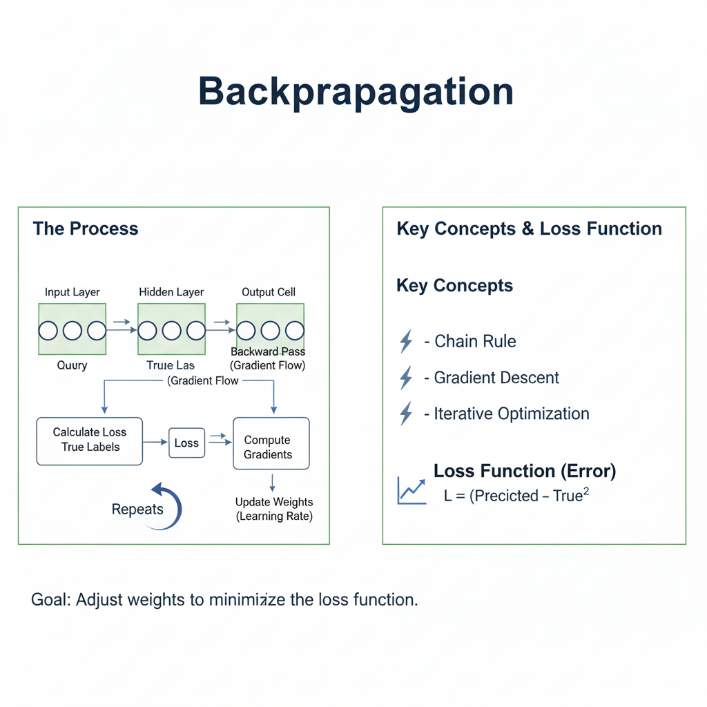
Often described as the “hidden engine” of deep learning, Backpropagation is the critical learning procedure that allows neural networks to learn from their mistakes. It is the mechanism by which a network adjusts its millions, or even trillions, of internal parameters (weights and biases) to minimize the difference between its predictions and the actual truth. Without Backpropagation, a neural network would be a static, non-adaptive function, incapable of the learning that defines modern AI.
While the models have grown exponentially more complex—from simple perceptrons to today’s massive transformer-based architectures—the core principle of Backpropagation has remained unchanged. It is a testament to the algorithm’s elegance and power. For anyone seeking to truly understand, debug, or advance AI systems in 2025, moving beyond a black-box understanding to master Backpropagation is not just beneficial—it is essential. This guide will demystify this core algorithm, taking you from its intuitive foundations to its practical implementation and its role in the cutting-edge AI of today.
Part 1: The “Why” – The Fundamental Problem of Learning
Before diving into the “how,” it’s crucial to understand the “why.” What problem does Backpropagation solve?
1.1 The Optimization Landscape
Imagine you are blindfolded on a mountainous landscape, and your goal is to find the lowest valley (the global minimum). You can’t see the entire landscape, but you can feel the steepness of the ground beneath your feet. The fundamental problem of training a neural network is analogous: we have a “loss function”—a mathematical representation of the model’s error—that forms a complex, high-dimensional landscape. Our goal is to find the set of weights that places us at the lowest point of this landscape.
How do we do this? We use the feeling of the steepness—the gradient. The gradient is a vector that points in the direction of the steepest ascent. Therefore, the negative of the gradient points in the direction of the steepest descent. Backpropagation is the highly efficient algorithm for calculating this gradient for every weight in the network.
1.2 The Chain Rule: The Mathematical Heart
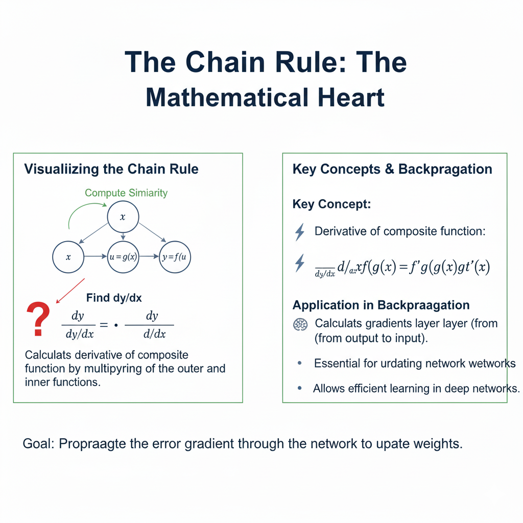
The conceptual leap at the core of Backpropagation is the application of the chain rule from calculus. A neural network is essentially a deeply nested function. The output is a function of the activations of the last layer, which are functions of the weights and activations of the previous layer, and so on, all the way back to the input.
The chain rule allows us to compute the derivative of the final loss with respect to a weight in the very first layer by breaking down the calculation into a series of simple derivatives. Backpropagation computes the gradient for the entire network in two passes:
- A forward pass to calculate the network’s output and the resulting loss.
- A backward pass to propagate the error gradient from the output layer back to the input layer, applying the chain rule at every step.
This is far more efficient than perturbing each weight individually to see its effect on the loss, a method that would be computationally impossible for modern networks with trillions of parameters.
Part 2: A Step-by-Step Walkthrough of the Algorithm
Let’s make this concrete by working through a simplified example: a network with two inputs, one hidden layer with two neurons, and one output.
Network Structure:
- Inputs: x1,x2x1,x2
- Hidden Layer: Neurons h1,h2h1,h2 with weights w1,1,w1,2,w2,1,w2,2w1,1,w1,2,w2,1,w2,2 and biases bh1,bh2bh1,bh2. We’ll use the Sigmoid activation function, σ(z)=11+e−zσ(z)=1+e−z1.
- Output Layer: Neuron ypredypred with weights v1,v2v1,v2 and bias bobo. We’ll use a linear activation for the output for simplicity.
- True Label: ytrueytrue
- Loss Function: Mean Squared Error, L=12(ytrue−ypred)2L=21(ytrue−ypred)2. The 1221 is a convenience that cancels out the exponent when we take the derivative.
Step 1: The Forward Pass
We calculate the output of the network step-by-step.
- Input to Hidden:
- zh1=w1,1×1+w2,1×2+bh1zh1=w1,1x1+w2,1x2+bh1
- zh2=w1,2×1+w2,2×2+bh2zh2=w1,2x1+w2,2x2+bh2
- ah1=σ(zh1)ah1=σ(zh1)
- ah2=σ(zh2)ah2=σ(zh2)
- Hidden to Output:
- zo=v1ah1+v2ah2+bozo=v1ah1+v2ah2+bo
- ypred=zoypred=zo (linear activation)
- Calculate Loss:
- L=12(ytrue−ypred)2L=21(ytrue−ypred)2
The forward pass gives us our current prediction and how wrong we are.
Step 2: The Backward Pass (Backpropagation)
This is where we calculate the gradient for every parameter. We work backwards from the loss.
- Gradient at the Output Layer:
We need ∂L∂v1∂v1∂L, ∂L∂v2∂v2∂L, and ∂L∂bo∂bo∂L. Let’s start with ∂L∂v1∂v1∂L. Using the chain rule:
∂L∂v1=∂L∂ypred⋅∂ypred∂zo⋅∂zo∂v1∂v1∂L=∂ypred∂L⋅∂zo∂ypred⋅∂v1∂zo- ∂L∂ypred=∂∂ypred(12(ytrue−ypred)2)=−(ytrue−ypred)∂ypred∂L=∂ypred∂(21(ytrue−ypred)2)=−(ytrue−ypred)
- ∂ypred∂zo=1∂zo∂ypred=1 (because of linear activation)
- ∂zo∂v1=ah1∂v1∂zo=ah1
- ∂L∂v1=δo⋅ah1∂v1∂L=δo⋅ah1
- ∂L∂v2=δo⋅ah2∂v2∂L=δo⋅ah2
- ∂L∂bo=δo⋅1=δo∂bo∂L=δo⋅1=δo (because zo=…+bozo=…+bo, so ∂zo∂bo=1∂bo∂zo=1)
- Gradient at the Hidden Layer:
Now, we move backward to find the gradients for the weights and biases in the hidden layer, e.g., ∂L∂w1,1∂w1,1∂L. The path of influence is longer:
w1,1→zh1→ah1→zo→Lw1,1→zh1→ah1→zo→LSo, ∂L∂w1,1=∂L∂zo⋅∂zo∂ah1⋅∂ah1∂zh1⋅∂zh1∂w1,1∂w1,1∂L=∂zo∂L⋅∂ah1∂zo⋅∂zh1∂ah1⋅∂w1,1∂zh1We already know ∂L∂zo=δo∂zo∂L=δo.- ∂zo∂ah1=v1∂ah1∂zo=v1
- ∂ah1∂zh1=σ(zh1)(1−σ(zh1))∂zh1∂ah1=σ(zh1)(1−σ(zh1)) (This is the derivative of the sigmoid function)
- ∂zh1∂w1,1=x1∂w1,1∂zh1=x1
δh1=∂L∂zh1=δo⋅v1⋅σ′(zh1)δh1=∂zh1∂L=δo⋅v1⋅σ′(zh1)This pattern is key to Backpropagation: the error signal for a layer is a weighted sum of the error signals from the next layer, multiplied by the derivative of the current layer’s activation function. This allows the error to flow backwards efficiently.- ∂L∂w1,1=δh1⋅x1∂w1,1∂L=δh1⋅x1
- ∂L∂bh1=δh1⋅1=δh1∂bh1∂L=δh1⋅1=δh1
Step 3: The Weight Update
Once we have all the gradients, we update the weights using Gradient Descent. For a weight ww, the update rule is:
wnew=wold−η⋅∂L∂woldwnew=wold−η⋅∂wold∂L
where ηη is the learning rate, a hyperparameter that controls the size of the step we take.
This entire process—forward pass, backward pass, weight update—is repeated for thousands or millions of iterations until the model converges to a good set of weights.
Part 3: Implementing Backpropagation from Scratch in Python (2025-Ready)
While modern deep learning frameworks like TensorFlow and PyTorch automate differentiation (a concept known as autograd), implementing Backpropagation from scratch is the best way to achieve true mastery. Here’s a clean, object-oriented implementation for a fully connected network.
python
import numpy as np
import matplotlib.pyplot as plt

class NeuralNetwork:
    """
    A fully connected neural network with manual backpropagation implementation.
    """
    def __init__(self, layer_sizes, learning_rate=0.1, activation='relu'):
        self.layer_sizes = layer_sizes
        self.learning_rate = learning_rate
        self.activation_name = activation

        # Initialize weights and biases using He initialization (good for ReLU)
        self.weights = []
        self.biases = []

        for i in range(len(layer_sizes) - 1):
            # He initialization: sqrt(2 / fan_in)
            fan_in = layer_sizes[i]
            weight_matrix = np.random.randn(layer_sizes[i+1], layer_sizes[i]) * np.sqrt(2. / fan_in)
            bias_vector = np.zeros((layer_sizes[i+1], 1))

            self.weights.append(weight_matrix)
            self.biases.append(bias_vector)

        # Cache for storing forward pass values for backpropagation
        self.cache = {}

    def _activation(self, z, derivative=False):
        """Apply activation function and its derivative."""
        if self.activation_name == 'relu':
            if derivative:
                return np.where(z > 0, 1.0, 0.0)
            return np.maximum(0, z)
        elif self.activation_name == 'sigmoid':
            s = 1 / (1 + np.exp(-z))
            if derivative:
                return s * (1 - s)
            return s
        elif self.activation_name == 'tanh':
            t = np.tanh(z)
            if derivative:
                return 1 - t**2
            return t
        elif self.activation_name == 'swish':  # 2025 Modern default
            s = 1 / (1 + np.exp(-z))
            if derivative:
                return s + z * s * (1 - s)
            return z * s

    def forward(self, X):
        """Perform forward pass through the network."""
        # Input layer
        A = X.T  # Transpose to (features, batch_size)
        self.cache['A0'] = A

        # Hidden layers
        for i in range(len(self.weights) - 1):
            Z = self.weights[i] @ A + self.biases[i]
            A = self._activation(Z)
            self.cache[f'Z{i+1}'] = Z
            self.cache[f'A{i+1}'] = A

        # Output layer (linear activation for regression, softmax for classification would go here)
        Z_out = self.weights[-1] @ A + self.biases[-1]
        A_out = Z_out  # Linear activation
        self.cache[f'Z{len(self.weights)}'] = Z_out
        self.cache[f'A{len(self.weights)}'] = A_out

        return A_out.T  # Transpose back to (batch_size, features)

    def backward(self, X, y, y_pred):
        """Perform backward pass to compute gradients."""
        m = X.shape[0]  # batch size
        gradients_w = [np.zeros_like(w) for w in self.weights]
        gradients_b = [np.zeros_like(b) for b in self.biases]

        # Calculate initial error (derivative of MSE loss)
        dA = (y_pred - y).T / m  # (output_size, batch_size)

        # Backpropagate through layers in reverse
        for l in range(len(self.weights)-1, -1, -1):
            if l == len(self.weights) - 1:
                # Output layer (linear activation)
                dZ = dA  # For linear activation, derivative is 1
                A_prev = self.cache[f'A{l}']
            else:
                # Hidden layers
                Z_curr = self.cache[f'Z{l+1}']
                dZ = dA * self._activation(Z_curr, derivative=True)
                A_prev = self.cache[f'A{l}']

            # Compute gradients for weights and biases at this layer
            gradients_w[l] = dZ @ A_prev.T
            gradients_b[l] = np.sum(dZ, axis=1, keepdims=True)

            # Compute gradient for next layer (if not at input)
            if l > 0:
                dA = self.weights[l].T @ dZ

        return gradients_w, gradients_b

    def update_parameters(self, gradients_w, gradients_b):
        """Update weights and biases using gradient descent."""
        for i in range(len(self.weights)):
            self.weights[i] -= self.learning_rate * gradients_w[i]
            self.biases[i] -= self.learning_rate * gradients_b[i]

    def train(self, X, y, epochs=1000, verbose=True):
        """Train the network using backpropagation."""
        losses = []

        for epoch in range(epochs):
            # Forward pass
            y_pred = self.forward(X)

            # Compute loss (Mean Squared Error)
            loss = np.mean((y_pred - y) ** 2)
            losses.append(loss)

            # Backward pass
            gradients_w, gradients_b = self.backward(X, y, y_pred)

            # Update parameters
            self.update_parameters(gradients_w, gradients_b)

            if verbose and epoch % (epochs // 10) == 0:
                print(f"Epoch {epoch}, Loss: {loss:.6f}")

        return losses

# Demonstration: Learn a simple non-linear function
if __name__ == "__main__":
    # Generate synthetic data: y = x^2 + noise
    np.random.seed(42)
    X_train = np.linspace(-2, 2, 100).reshape(-1, 1)
    y_train = X_train**2 + np.random.normal(0, 0.1, X_train.shape)

    print("Creating and training neural network...")
    # Network architecture: 1 input -> 64 hidden (ReLU) -> 32 hidden (ReLU) -> 1 output (Linear)
    nn = NeuralNetwork(layer_sizes=[1, 64, 32, 1], learning_rate=0.01, activation='relu')

    # Train the network
    losses = nn.train(X_train, y_train, epochs=5000, verbose=True)

    # Test the network
    X_test = np.linspace(-2, 2, 50).reshape(-1, 1)
    y_pred = nn.forward(X_test)

    # Plot results
    plt.figure(figsize=(12, 5))

    plt.subplot(1, 2, 1)
    plt.scatter(X_train, y_train, alpha=0.7, label='Training Data', s=20)
    plt.plot(X_test, y_pred, 'r-', linewidth=2, label='Network Prediction')
    plt.plot(X_test, X_test**2, 'g--', alpha=0.8, label='True Function (x²)')
    plt.xlabel('x')
    plt.ylabel('y')
    plt.title('Function Approximation with Backpropagation')
    plt.legend()
    plt.grid(True, alpha=0.3)

    plt.subplot(1, 2, 2)
    plt.plot(losses)
    plt.xlabel('Epoch')
    plt.ylabel('Mean Squared Error Loss')
    plt.title('Training Loss Over Time')
    plt.yscale('log')
    plt.grid(True, alpha=0.3)

    plt.tight_layout()
    plt.show()

    print(f"\nFinal training loss: {losses[-1]:.6f}")
Part 4: Backpropagation in the Age of Autograd and LLMs (2025 Context)
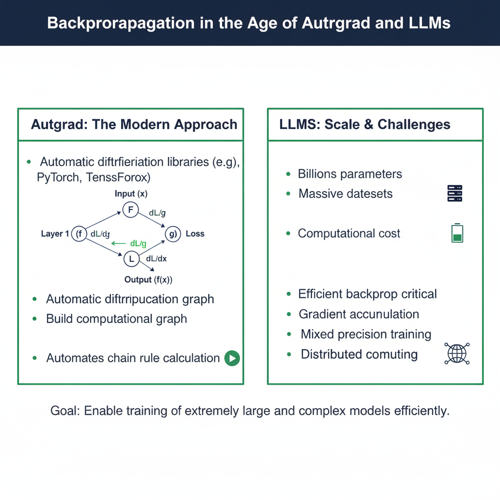
In 2025, you will almost never implement Backpropagation manually for production models. So, why is mastering it still crucial?
4.1 Understanding Automatic Differentiation (Autograd)
Frameworks like PyTorch and TensorFlow use automatic differentiation. When you define a computation (a forward pass), the framework builds a computational graph. During the backward pass, it automatically applies the chain rule to compute gradients.
python
# PyTorch-like autograd example
import torch

x = torch.tensor([1.0, 2.0], requires_grad=True)
w = torch.tensor([0.5, -0.3], requires_grad=True)
b = torch.tensor(0.1, requires_grad=True)

# Forward pass
z = torch.dot(w, x) + b
y = torch.sigmoid(z)
loss = (y - 1.0) ** 2

# Backward pass (PyTorch automatically computes gradients!)
loss.backward()

print(f"Gradient of loss w.r.t w: {w.grad}")  # Autograd computes this via backpropagation
print(f"Gradient of loss w.r.t b: {b.grad}")
Mastering Backpropagation allows you to understand what autograd is doing, which is essential for debugging and creating custom operations.
4.2 The Scale of Modern Backpropagation
Large Language Models (LLMs) like GPT-4 represent the ultimate scaling of Backpropagation. The algorithm remains the same, but the engineering challenge is monumental.
- Trillions of Parameters: Calculating and storing gradients for trillions of weights requires sophisticated model parallelism and memory optimization techniques.
- Distributed Training: Backpropagation is performed across thousands of GPUs simultaneously, with gradients being synchronized across all devices.
- Memory Management: Techniques like gradient checkpointing (recomputing some activations during the backward pass instead of storing them) are used to fit massive models into GPU memory.
Part 5: Advanced Topics and Common Challenges
5.1 The Vanishing/Exploding Gradient Problem
This is a fundamental challenge in deep networks. During Backpropagation, as the error signal is propagated backwards, it is multiplied by the weight matrices and the derivatives of the activation functions repeatedly. If these values are consistently less than 1, the gradient can vanish (become infinitesimally small). If they are greater than 1, it can explode.
2025 Solutions:
- Architectural Choices: Using Residual Connections (from ResNet) and Skip Connections provides a “highway” for the gradient to flow directly backwards, mitigating vanishing gradients.
- Normalization Layers: Batch Normalization and Layer Normalization stabilize the distributions of layer inputs, which in turn stabilizes gradient flow.
- Activation Functions: The switch from Sigmoid/Tanh to ReLU and its variants (Leaky ReLU, Swish) was largely driven by their more stable derivatives, which are less prone to vanishing.
5.2 Second-Order Optimization Methods
While basic Gradient Descent uses only the first derivative (gradient), more advanced optimizers like Adam, AdamW (the 2025 standard), and LAMB incorporate concepts from second-order optimization. They estimate a per-parameter learning rate by tracking not just the gradient but also its second moment (uncentered variance). Understanding Backpropagation is the prerequisite for understanding these advanced optimizers.
Conclusion: The Unchanging Engine in an Evolving Field
Backpropagation is the bedrock upon which the modern AI revolution is built. From the simplest logistic regression model to the most complex trillion-parameter transformer, the same core algorithm—the efficient computation of gradients via the chain rule—enables learning.
Mastering Backpropagation in 2025 provides you with:
- Deep Intuition: The ability to look at any neural architecture and understand its learning dynamics.
- Debugging Power: When a model fails to train, knowledge of Backpropagation is your most powerful tool for diagnosing whether the issue is vanishing gradients, improper initialization, or a software bug.
- Innovation Capacity: It allows you to move beyond using existing layers to designing new ones, confident that you can compute the necessary gradients.
As AI continues its rapid advance, the principles of Backpropagation will remain constant. It is the hidden engine that, once mastered, turns the black box of deep learning into a transparent, understandable, and powerful tool for creation.