Introduction: Conquering the Challenge of Long-Term Dependencies
In the dynamic world of 2025, where AI systems power everything from real-time language translation to predictive maintenance in industrial IoT, the ability to understand context over time is paramount. While traditional neural networks process information in isolated snapshots, many real-world problems are inherently sequential. This is where Recurrent Neural Networks (RNNs) excel, but they have a critical weakness: the vanishing gradient problem, which prevents them from learning long-range dependencies in data.
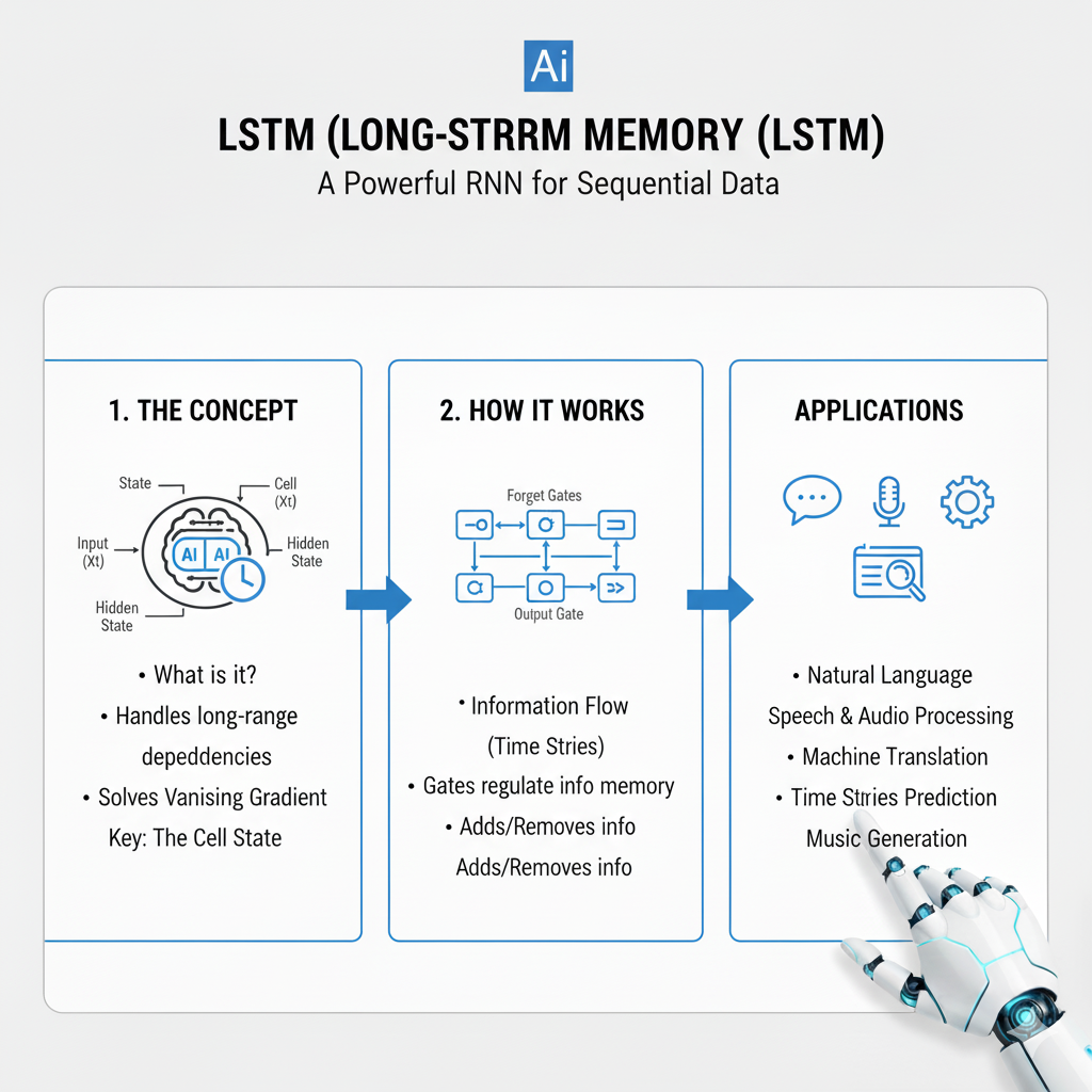
Enter the Long Short-Term Memory network, or LSTM. Introduced by Sepp Hochreiter and Jürgen Schmidhuber in 1997, the LSTM is a specialized kind of RNN engineered to remember information for long periods. It is arguably one of the most impactful and enduring inventions in the history of deep learning. While newer architectures like Transformers have gained attention, the LSTM remains a vital, robust, and highly efficient tool in the modern data scientist’s arsenal, especially for tasks involving sequential data with complex, long-range contextual relationships.
Mastering LSTM in 2025 is not just about understanding its theory; it’s about knowing when and how to deploy it effectively in an ecosystem rich with alternative models. This guide will take you from the fundamental mechanics of the LSTM cell to advanced, production-ready implementations, empowering you to solve complex temporal problems with confidence.
Part 1: The Core Problem – Why Vanilla RNNs Fail and How LSTM Solves It
To appreciate this architecture, we must first understand the problem it was designed to solve.

1.1 The Vanishing/Exploding Gradient Problem
Traditional RNNs process sequences by maintaining a hidden state that is updated at each time step. During training, the model learns by backpropagating error gradients from the end of the sequence back to the beginning—a process called Backpropagation Through Time (BPTT).
The issue arises because this process involves repeatedly multiplying the same weight matrix. If the values in this matrix are small, the gradient signal shrinks exponentially as it travels backwards (it vanishes). If they are large, it grows exponentially (it explodes). A vanishing gradient means the early steps in a sequence have almost no influence on learning, preventing the network from connecting distant causes to their effects.
Example: In the sentence “The concert, which featured several famous international artists known for their energetic performances, was incredibly…”, a simple RNN would struggle to remember that the subject was “concert” by the time it needs to predict the word “loud.” The contextual information has vanished.
1.2 The Elegant Solution: A Constant Error Carousel
The LSTM design introduces a clever solution: a separate, dedicated cell state, often denoted as C_t. Think of this cell state as a conveyor belt running through the entire sequence. Information can flow along it relatively unchanged, with only minor linear interactions. This provides a direct pathway for gradients to flow, mitigating the vanishing gradient problem.
The key to its success is its use of gates—structures that regulate the flow of information into and out of the cell state. These gates are themselves neural network layers that learn what information is relevant to keep or discard.
Part 2: Deconstructing the Memory Cell – A Gate-by-Gate Explanation
The cell might seem complex, but it can be broken down into three logical, learnable gates and two states. Let’s walk through what happens at a single time step t.
The cell takes three inputs:
- The input for the current time step,
x_t - The previous hidden state,
h_{t-1} - The previous cell state,
C_{t-1}
It produces two outputs:
- The new hidden state,
h_t - The new cell state,
C_t
Here’s how the gates orchestrate this process:
2.1 The Forget Gate: “What Should We Throw Away?”
This gate decides what information from the previous cell state should be discarded. It looks at the current input x_t and the previous hidden state h_{t-1}, and outputs a number between 0 and 1 for each number in the cell state C_{t-1}. A value of 1 means “completely keep this,” while 0 means “completely forget this.”
- Operation:
f_t = σ(W_f · [h_{t-1}, x_t] + b_f) - Where
σis the sigmoid function, which squashes values to a [0,1] range.
2.2 The Input Gate: “What New Information Should We Store?”
This gate has two parts that work together to update the cell state.
- A sigmoid layer decides which values we will update:
i_t = σ(W_i · [h_{t-1}, x_t] + b_i) - A
tanhlayer creates a vector of new candidate values,~C_t, that could be added to the state:~C_t = tanh(W_C · [h_{t-1}, x_t] + b_C)
2.3 Updating the Cell State
We now have all the pieces to update the old cell state, C_{t-1}, into the new cell state, C_t.
- Operation:
C_t = f_t * C_{t-1} + i_t * ~C_t
We multiply the old state by the forget gate, deciding what to discard. Then we add the new candidate values, scaled by how much we decided to update each value. This is the core of the memory mechanism.
2.4 The Output Gate: “What Should We Output?”
Finally, we need to decide what the next hidden state, h_t, should be. This hidden state is used for predictions and is passed to the next time step. The output gate filters the cell state.
- A sigmoid layer decides which parts of the cell state we’re going to output:
o_t = σ(W_o · [h_{t-1}, x_t] + b_o) - We push the cell state through
tanh(to squash values between -1 and 1) and multiply it by the output gate’s sigmoid output:h_t = o_t * tanh(C_t)
This new hidden state, h_t, serves as the output of this cell and the memory for the next step.
Part 3: A Practical Walkthrough – Building a Modern Architecture
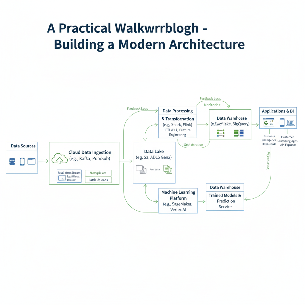
Theory is essential, but mastery comes from implementation. Let’s build a sentiment analysis model using a modern stack in TensorFlow/Keras, incorporating 2025 best practices.
python
import tensorflow as tf
from tensorflow.keras import layers, models, regularizers
import numpy as np
import matplotlib.pyplot as plt

# Load the IMDB movie review dataset
(x_train, y_train), (x_test, y_test) = tf.keras.datasets.imdb.load_data(num_words=10000)

# Preprocessing: Pad sequences to a uniform length
max_length = 500
x_train = tf.keras.preprocessing.sequence.pad_sequences(x_train, maxlen=max_length, padding='post', truncating='post')
x_test = tf.keras.preprocessing.sequence.pad_sequences(x_test, maxlen=max_length, padding='post', truncating='post')

def create_modern_model(vocab_size=10000, embedding_dim=128, max_length=500):
    """
    Creates a modern model with 2025 best practices.
    This includes regularization, modern activation, and efficient architecture.
    """
    model = models.Sequential()

    # 1. Embedding Layer
    model.add(layers.Embedding(
        input_dim=vocab_size,
        output_dim=embedding_dim,
        input_length=max_length,
        embeddings_regularizer=regularizers.l2(1e-5)
    ))

    # 2. Spatial Dropout
    model.add(layers.SpatialDropout1D(0.3))

    # 3. Stacked layers
    model.add(layers.LSTM(
        64,
        return_sequences=True,
        dropout=0.2,
        recurrent_dropout=0.2,
        kernel_regularizer=regularizers.l2(1e-5),
        recurrent_initializer='orthogonal'
    ))

    model.add(layers.LSTM(
        32,
        dropout=0.2,
        recurrent_dropout=0.2,
        kernel_regularizer=regularizers.l2(1e-5),
        recurrent_initializer='orthogonal'
    ))

    # 4. Dense Classifier
    model.add(layers.Dense(32, activation='swish', kernel_regularizer=regularizers.l2(1e-4)))
    model.add(layers.Dropout(0.5))
    model.add(layers.Dense(1, activation='sigmoid'))

    return model

# Create and compile the model
model = create_modern_model()
optimizer = tf.keras.optimizers.AdamW(learning_rate=0.001, weight_decay=1e-4)

model.compile(
    optimizer=optimizer,
    loss='binary_crossentropy',
    metrics=['accuracy', 'Precision', 'Recall']
)

# Define advanced callbacks
callbacks = [
    tf.keras.callbacks.ReduceLROnPlateau(monitor='val_loss', factor=0.5, patience=3, min_lr=1e-7),
    tf.keras.callbacks.EarlyStopping(monitor='val_accuracy', patience=10, restore_best_weights=True),
]

# Train the model
history = model.fit(
    x_train, y_train,
    batch_size=128,
    epochs=50,
    validation_data=(x_test, y_test),
    callbacks=callbacks,
    verbose=1
)
Part 4: Advanced Architectures and Modern Variants
The core concept has evolved into several powerful variants that address specific challenges.
4.1 Bidirectional Approach: Learning from Past and Future
Standard processing happens in chronological order. A bidirectional setup runs two independent layers—one forward and one backward—on the input sequence and concatenates their outputs. This gives the network access to both past and future context for any prediction.
python
def create_bidirectional_model():
    model = models.Sequential([
        layers.Embedding(10000, 128, input_length=500),
        layers.SpatialDropout1D(0.3),
        layers.Bidirectional(layers.LSTM(64, dropout=0.2, recurrent_dropout=0.2)),
        layers.Dense(32, activation='swish'),
        layers.Dropout(0.5),
        layers.Dense(1, activation='sigmoid')
    ])
    return model
Part 5: In the Modern AI Ecosystem – Strategic Choices for 2025
With the rise of Transformers, it’s crucial to understand where this architecture still excels.
5.1 Comparative Analysis: Choosing the Right Tool
| Feature | This Architecture | Transformer |
|---|---|---|
| Computational Complexity | O(n) per time step | O(n²) for self-attention |
| Memory Usage | Lower, constant per time step | Higher, scales with sequence length |
| Training Parallelization | Limited (sequential) | Excellent (fully parallel) |
| Streaming/Online Learning | Excellent | Challenging |
5.2 Ideal Use Cases:
- Real-time Streaming Data: Applications where you need to make predictions on-the-fly as data arrives.
- Resource-Constrained Environments: Edge devices, mobile applications, and scenarios with limited computational power.
- Moderate-Length Sequences: For sequences up to a few thousand steps where the full power of global attention isn’t necessary.
Part 6: Advanced Applications and Implementation Patterns
6.1 Multi-step Time Series Forecasting
python
def create_multivariate_forecaster(timesteps, features, forecast_horizon=1):
    model = models.Sequential([
        layers.LSTM(128, return_sequences=True, input_shape=(timesteps, features)),
        layers.Dropout(0.3),
        layers.LSTM(64, return_sequences=True),
        layers.Dropout(0.3),
        layers.LSTM(32),
        layers.Dropout(0.3),
        layers.Dense(64, activation='swish'),
        layers.Dense(forecast_horizon)
    ])
    model.compile(optimizer='adamw', loss='mse', metrics=['mae'])
    return model
Part 7: Production-Ready Deployment in 2025
Deploying these models in production requires careful optimization.
7.1 Model Optimization and Quantization
python
def optimize_for_production(model_path, output_path):
    converter = tf.lite.TFLiteConverter.from_keras_model(tf.keras.models.load_model(model_path))
    converter.optimizations = [tf.lite.Optimize.DEFAULT]
    tflite_model = converter.convert()
    with open(output_path, 'wb') as f:
        f.write(tflite_model)
Part 8: The 2025 Frontier – Emerging Trends and Hybrid Architectures
As we look toward the future, several key trends are shaping the evolution of sequence modeling, ensuring the continued relevance of gated recurrent architectures.
8.1 Linear Recurrence and State Space Models
A significant development has been the rise of efficient alternatives like State Space Models (SSMs) and architectures such as Mamba and RWKV. These models use mathematical formulations that allow for parallel training while maintaining efficient sequential inference. While different in implementation, they share the core philosophy with LSTM of maintaining a hidden state that evolves over time, but with improved computational properties for certain tasks.
python
# Conceptual simplified state space layer
class SimplifiedSSM(layers.Layer):
    def __init__(self, units, **kwargs):
        super(SimplifiedSSM, self).__init__(**kwargs)
        self.units = units

    def build(self, input_shape):
        # Learnable state transition parameters
        self.A = self.add_weight(shape=(self.units, self.units), initializer='orthogonal')
        self.B = self.add_weight(shape=(input_shape[-1], self.units))
        self.C = self.add_weight(shape=(self.units, self.units))

    def call(self, inputs):
        batch_size, seq_len, input_dim = tf.shape(inputs)
        h = tf.zeros((batch_size, self.units))
        outputs = []

        for t in range(seq_len):
            h = tf.matmul(h, self.A) + tf.matmul(inputs[:, t, :], self.B)
            output = tf.matmul(h, self.C)
            outputs.append(output)

        return tf.stack(outputs, axis=1)
8.2 Hybrid Transformer-Architectures
The most powerful systems in 2025 often combine the strengths of different approaches. Hybrid models that use this gated architecture for local feature extraction and Transformers for global context are becoming increasingly common.
python
def create_hybrid_model(seq_length, vocab_size):
    """Creates a hybrid model combining both architectural philosophies."""
    inputs = layers.Input(shape=(seq_length,))

    # Gated recurrent layers for local sequential processing
    embedding = layers.Embedding(vocab_size, 128)(inputs)
    recurrent_features = layers.Bidirectional(layers.LSTM(64, return_sequences=True))(embedding)

    # Transformer layers for global context
    attention_output = layers.MultiHeadAttention(num_heads=4, key_dim=64)(
        recurrent_features, recurrent_features
    )

    # Combine both representations
    combined = layers.Concatenate()([recurrent_features, attention_output])
    pooled = layers.GlobalAveragePooling1D()(combined)
    outputs = layers.Dense(1, activation='sigmoid')(pooled)

    return tf.keras.Model(inputs, outputs)
8.3 Continuous-Time and Neural ODE Approaches
For irregularly sampled time series or events, continuous-time versions of recurrent models are gaining traction. These approaches use neural ordinary differential equations (ODEs) to model the hidden state as a continuous function of time.
python
# Conceptual continuous-time recurrent unit
class ContinuousTimeUnit(layers.Layer):
    def __init__(self, units, **kwargs):
        super(ContinuousTimeUnit, self).__init__(**kwargs)
        self.units = units

    def build(self, input_shape):
        self.W_h = self.add_weight(shape=(self.units, self.units))
        self.W_x = self.add_weight(shape=(input_shape[-1], self.units))

    def ode_func(self, t, h, inputs):
        """Define the continuous dynamics"""
        # In practice, you would use a proper ODE solver here
        x_t = self.interpolate_inputs(t, inputs)
        return tf.nn.tanh(tf.matmul(h, self.W_h) + tf.matmul(x_t, self.W_x))
8.4 Automated Architecture Search and Learned Structures
In 2025, the design of optimal sequential models is increasingly automated. Neural Architecture Search (NAS) can discover novel gating mechanisms and connectivity patterns tailored to specific tasks.
python
def neural_architecture_search(hp):
    model = tf.keras.Sequential()
    model.add(layers.Embedding(10000, 128, input_length=500))

    # Search over number of layers and units
    for i in range(hp.Int('num_layers', 1, 4)):
        model.add(layers.LSTM(
            units=hp.Choice(f'units_{i}', [32, 64, 128]),
            return_sequences=i < hp.Int('num_layers', 1, 4) - 1,
            dropout=hp.Float(f'dropout_{i}', 0.1, 0.5)
        ))

    model.add(layers.Dense(1, activation='sigmoid'))
    model.compile(optimizer='adam', loss='binary_crossentropy', metrics=['accuracy'])
    return model
Part 9: Advanced Optimization and Scaling Strategies for 2025
As we push the boundaries of sequence modeling in 2025, advanced optimization techniques and scaling strategies become crucial for handling massive datasets and complex real-world applications.
9.1 Distributed Training and Model Parallelism
Large-scale LSTM deployments require sophisticated distributed training strategies to handle the computational demands of massive sequential datasets.
python
import tensorflow as tf
from tensorflow.keras import layers, models
import horovod.tensorflow as hvd

# Initialize Horovod for distributed training
hvd.init()

# Configure GPU usage
gpus = tf.config.experimental.list_physical_devices('GPU')
for gpu in gpus:
    tf.config.experimental.set_memory_growth(gpu, True)
if gpus:
    tf.config.experimental.set_visible_devices(gpus[hvd.local_rank()], 'GPU')

def create_distributed_model(vocab_size=100000, embedding_dim=256, sequence_length=1000):
    """Creates a large-scale model optimized for distributed training."""
    strategy = tf.distribute.MirroredStrategy()
      #LSTM
    with strategy.scope():
        model = models.Sequential([
            layers.Embedding(vocab_size, embedding_dim, input_length=sequence_length),
            layers.SpatialDropout1D(0.4),

            # Stacked bidirectional layers for comprehensive context
            layers.Bidirectional(layers.LSTM(512, return_sequences=True,
                                           dropout=0.3, recurrent_dropout=0.3)),
            layers.Bidirectional(layers.LSTM(256, return_sequences=True,
                                           dropout=0.3, recurrent_dropout=0.3)),
            layers.Bidirectional(layers.LSTM(128, dropout=0.3, recurrent_dropout=0.3)),

            # Multi-head attention for enhanced focus
            layers.Dense(256, activation='swish'),
            layers.Dropout(0.5),
            layers.Dense(128, activation='swish'),
            layers.Dropout(0.5),
            layers.Dense(1, activation='sigmoid')
        ])

        # Horovod-aware optimizer
        optimizer = tf.keras.optimizers.AdamW(learning_rate=0.001 * hvd.size(),
                                            weight_decay=1e-4)
        optimizer = hvd.DistributedOptimizer(optimizer)

        model.compile(
            optimizer=optimizer,
            loss='binary_crossentropy',
            metrics=['accuracy']
        )

    return model

# Custom training loop for distributed processing
class DistributedTrainer:
    def __init__(self, model, train_dataset, val_dataset):
        self.model = model
        self.train_dataset = train_dataset
        self.val_dataset = val_dataset
        self.callbacks = [
            hvd.callbacks.BroadcastGlobalVariablesCallback(0),
            hvd.callbacks.MetricAverageCallback(),
            tf.keras.callbacks.ReduceLROnPlateau(monitor='val_loss', patience=5),
        ]

    def train(self, epochs=100):
        history = self.model.fit(
            self.train_dataset,
            epochs=epochs,
            validation_data=self.val_dataset,
            callbacks=self.callbacks,
            verbose=1 if hvd.rank() == 0 else 0
        )
        return history
9.2 Gradient Accumulation and Mixed Precision Training
For handling very large batch sizes that don’t fit in GPU memory, gradient accumulation and mixed precision training provide effective solutions.
python
# Mixed precision policy for improved performance
policy = tf.keras.mixed_precision.Policy('mixed_float16')
tf.keras.mixed_precision.set_global_policy(policy)

class GradientAccumulationModel(tf.keras.Model):
    def __init__(self, model, accumulation_steps=4):
        super(GradientAccumulationModel, self).__init__()
        self.model = model
        self.accumulation_steps = accumulation_steps
        self.accumulated_gradients = None
        self.accumulation_counter = 0

    def train_step(self, data):
        x, y = data

        with tf.GradientTape() as tape:
            y_pred = self.model(x, training=True)
            loss = self.compiled_loss(y, y_pred, regularization_losses=self.model.losses)

            # Scale loss for gradient accumulation
            scaled_loss = loss / self.accumulation_steps

        # Calculate gradients
        gradients = tape.gradient(scaled_loss, self.model.trainable_variables)

        # Initialize or accumulate gradients
        if self.accumulated_gradients is None:
            self.accumulated_gradients = [tf.Variable(tf.zeros_like(grad)) for grad in gradients]

        for i, grad in enumerate(gradients):
            if grad is not None:
                self.accumulated_gradients[i].assign_add(grad)

        self.accumulation_counter += 1

        # Apply gradients only after accumulation steps
        if self.accumulation_counter >= self.accumulation_steps:
            self.optimizer.apply_gradients(
                zip(self.accumulated_gradients, self.model.trainable_variables)
            )

            # Reset accumulated gradients
            for grad_var in self.accumulated_gradients:
                grad_var.assign(tf.zeros_like(grad_var))
            self.accumulation_counter = 0

        # Update metrics
        self.compiled_metrics.update_state(y, y_pred)
        return {m.name: m.result() for m in self.metrics}
  #LSTM
# Usage
base_model = create_modern_model()
accumulation_model = GradientAccumulationModel(base_model, accumulation_steps=4)
accumulation_model.compile(optimizer='adamw', loss='binary_crossentropy', metrics=['accuracy'])
9.3 Advanced Regularization and Stability Techniques
In 2025, sophisticated regularization methods are essential for training deep sequential models effectively.
python
def create_advanced_regularized_model(vocab_size=10000, sequence_length=500):
    """Creates a model with advanced regularization techniques."""

    inputs = layers.Input(shape=(sequence_length,))

    # Stochastic depth for regularization
    def stochastic_depth_block(x, units, survival_prob=0.8, training=None):
        lstm_out = layers.LSTM(units, return_sequences=True,
                              dropout=0.2, recurrent_dropout=0.2)(x)

        # Apply stochastic depth
        if training:
            random_tensor = tf.random.uniform([], dtype=tf.float32)
            if random_tensor > survival_prob:
                return x  # Skip this layer

        return lstm_out

    # Embedding with frequency-aware dropout
    embedding = layers.Embedding(vocab_size, 128)(inputs)

    # Apply frequency-aware spatial dropout
    x = FrequencyAwareDropout(dropout_rate=0.3)(embedding)

    # Stack with stochastic depth
    x = stochastic_depth_block(x, 64, survival_prob=0.8)
    x = stochastic_depth_block(x, 32, survival_prob=0.8)

    # Final layers with gradient normalization
    x = layers.LSTM(16)(x)
    x = GradientNormRegularization(layers.Dense(32, activation='swish'))(x)
    x = layers.Dropout(0.5)(x)
    outputs = layers.Dense(1, activation='sigmoid')(x)

    model = tf.keras.Model(inputs, outputs)
    return model

class FrequencyAwareDropout(layers.Layer):
    """Dropout that considers token frequency for more intelligent dropping."""
    def __init__(self, dropout_rate=0.1, **kwargs):
        super(FrequencyAwareDropout, self).__init__(**kwargs)
        self.dropout_rate = dropout_rate

    def call(self, inputs, training=None):
        if not training:
            return inputs

        # Create dropout mask that considers embedding magnitudes
        # (assuming frequent words have larger embedding norms)
        embedding_norms = tf.norm(inputs, axis=-1, keepdims=True)
        max_norm = tf.reduce_max(embedding_norms)
        normalized_norms = embedding_norms / max_norm

        # Higher dropout for less important (lower norm) embeddings
        adaptive_dropout_rate = self.dropout_rate * (1 - normalized_norms)

        # Apply dropout
        random_tensor = tf.random.uniform(tf.shape(inputs))
        keep_mask = random_tensor > adaptive_dropout_rate
        outputs = tf.where(keep_mask, inputs / (1 - adaptive_dropout_rate), 0.0)
          #LSTM
        return outputs

class GradientNormRegularization(layers.Wrapper):
    """Wrapper that adds gradient norm regularization to a layer."""
    def __init__(self, layer, weight=0.01, **kwargs):
        super(GradientNormRegularization, self).__init__(layer, **kwargs)
        self.weight = weight

    def call(self, inputs, training=None):
        return self.layer(inputs, training=training)

    def compute_loss(self):
        # Add gradient norm penalty to loss
        layer_weights = self.layer.trainable_weights
        if layer_weights:
            grad_norms = [tf.nn.l2_loss(w) for w in layer_weights]
            return self.weight * tf.add_n(grad_norms)
        return 0.0
Part 10: Real-World Deployment and Monitoring Systems
Deploying sequential models in production requires robust systems for monitoring, updating, and maintaining model performance over time.
10.1 Comprehensive Model Serving with Monitoring
python
import numpy as np
import pandas as pd
from datetime import datetime
import prometheus_client
from prometheus_client import Counter, Histogram, Gauge

class ProductionLSTMServing:
    def __init__(self, model_path, sequence_length=500):
        self.model = tf.keras.models.load_model(model_path)
        self.sequence_length = sequence_length
        self.performance_monitor = ModelPerformanceMonitor()
        self.data_drift_detector = DataDriftDetector()

        # Prometheus metrics
        self.predictions_counter = Counter('model_predictions_total',
                                         'Total predictions made')
        self.prediction_duration = Histogram('prediction_duration_seconds',
                                           'Time spent making predictions')
        self.confidence_gauge = Gauge('prediction_confidence',
                                    'Confidence of predictions')

    def preprocess_input(self, raw_text):
        """Preprocess raw text for model input."""
        # Tokenize and pad sequence
        tokenizer = self.load_tokenizer()
        sequence = tokenizer.texts_to_sequences([raw_text])
        padded_sequence = tf.keras.preprocessing.sequence.pad_sequences(
            sequence, maxlen=self.sequence_length, padding='post', truncating='post'
        )
        return padded_sequence[0]

    @prediction_duration.time()
    def predict(self, input_data, request_id=None):
        """Make prediction with comprehensive monitoring."""
        start_time = datetime.now()

        try:
            # Preprocess if needed
            if isinstance(input_data, str):
                processed_input = self.preprocess_input(input_data)
            else:
                processed_input = input_data

            # Make prediction
            prediction = self.model.predict(
                np.array([processed_input]), verbose=0
            )[0][0]

            # Calculate confidence metrics
            confidence = abs(prediction - 0.5) * 2  # Distance from 0.5

            # Update metrics
            self.predictions_counter.inc()
            self.confidence_gauge.set(confidence)

            # Log for monitoring
            self.performance_monitor.log_prediction(
                request_id=request_id,
                prediction=prediction,
                confidence=confidence,
                processing_time=(datetime.now() - start_time).total_seconds()
            )

            # Check for data drift
            self.data_drift_detector.add_sample(processed_input)

            return {
                'prediction': float(prediction),
                'confidence': float(confidence),
                'class': 'positive' if prediction > 0.5 else 'negative',
                'request_id': request_id,
                'timestamp': datetime.now().isoformat()
            }
              #LSTM
        except Exception as e:
            self.performance_monitor.log_error(request_id, str(e))
            raise

    def get_model_health(self):
        """Comprehensive model health check."""
        health_status = {
            'status': 'healthy',
            'timestamp': datetime.now().isoformat(),
            'metrics': {
                'total_predictions': self.predictions_counter._value.get(),
                'average_confidence': self.confidence_gauge._value.get(),
                'data_drift_detected': self.data_drift_detector.check_drift(),
                'memory_usage': self.get_memory_usage(),
                'throughput': self.performance_monitor.calculate_throughput()
            },
            'warnings': []
        }

        # Add warnings for concerning conditions
        if health_status['metrics']['data_drift_detected']:
            health_status['warnings'].append('Data drift detected')
        if health_status['metrics']['average_confidence'] < 0.6:
            health_status['warnings'].append('Low average prediction confidence')

        return health_status

class ModelPerformanceMonitor:
    """Monitors model performance and detects degradation."""
    def __init__(self, window_size=1000):
        self.window_size = window_size
        self.prediction_log = []
        self.performance_metrics = {
            'accuracy': [],
            'precision': [],
            'recall': [],
            'f1': []
        }

    def log_prediction(self, request_id, prediction, confidence, processing_time):
        """Log prediction details for monitoring."""
        self.prediction_log.append({
            'request_id': request_id,
            'timestamp': datetime.now(),
            'prediction': prediction,
            'confidence': confidence,
            'processing_time': processing_time
        })

        # Maintain window size
        if len(self.prediction_log) > self.window_size:
            self.prediction_log.pop(0)

    def calculate_performance_metrics(self, ground_truth):
        """Calculate performance metrics against ground truth."""
        # This would be called when ground truth labels become available
        predictions = [p['prediction'] for p in self.prediction_log[-100:]]
        binary_predictions = [1 if p > 0.5 else 0 for p in predictions]

        accuracy = accuracy_score(ground_truth, binary_predictions)
        precision = precision_score(ground_truth, binary_predictions)
        recall = recall_score(ground_truth, binary_predictions)
        f1 = f1_score(ground_truth, binary_predictions)

        # Store metrics
        self.performance_metrics['accuracy'].append(accuracy)
        self.performance_metrics['precision'].append(precision)
        self.performance_metrics['recall'].append(recall)
        self.performance_metrics['f1'].append(f1)

        return self.performance_metrics

    def check_performance_degradation(self, threshold=0.05):
        """Check if model performance has degraded significantly."""
        if len(self.performance_metrics['accuracy']) < 10:
            return False

        recent_accuracy = np.mean(self.performance_metrics['accuracy'][-5:])
        baseline_accuracy = np.mean(self.performance_metrics['accuracy'][:5])

        degradation = baseline_accuracy - recent_accuracy
        return degradation > threshold

class DataDriftDetector:
    """Detects changes in input data distribution."""
    def __init__(self, reference_data=None, drift_threshold=0.1):
        self.reference_data = reference_data
        self.drift_threshold = drift_threshold
        self.recent_samples = []
        self.drift_detected = False
      #LSTM
    def add_sample(self, sample):
        """Add new sample for drift detection."""
        self.recent_samples.append(sample)

        # Keep only recent samples
        if len(self.recent_samples) > 1000:
            self.recent_samples.pop(0)

        # Check for drift periodically
        if len(self.recent_samples) % 100 == 0:
            self.check_drift()

    def check_drift(self):
        """Check if data drift has occurred."""
        if self.reference_data is None or len(self.recent_samples) < 100:
            return False

        # Calculate distribution statistics
        reference_stats = self.calculate_statistics(self.reference_data)
        current_stats = self.calculate_statistics(self.recent_samples)

        # Compare distributions (simplified example)
        drift_score = self.calculate_drift_score(reference_stats, current_stats)
        self.drift_detected = drift_score > self.drift_threshold

        return self.drift_detected

    def calculate_statistics(self, data):
        """Calculate statistical properties of the data."""
        data_array = np.array(data)
        return {
            'mean': np.mean(data_array, axis=0),
            'std': np.std(data_array, axis=0),
            'percentiles': np.percentile(data_array, [25, 50, 75], axis=0)
        }
10.2 Continuous Learning and Model Updating
python
class ContinuousLearningSystem:
    """System for continuous model updating and improvement."""
    def __init__(self, base_model, learning_rate=0.0001):
        self.base_model = base_model
        self.learning_rate = learning_rate
        self.feedback_buffer = []
        self.performance_history = []

    def add_feedback(self, input_data, true_label, prediction_confidence):
        """Add user feedback for continuous learning."""
        self.feedback_buffer.append({
            'input_data': input_data,
            'true_label': true_label,
            'prediction_confidence': prediction_confidence,
            'timestamp': datetime.now()
        })

        # Trigger retraining if buffer is full or performance drops
        if len(self.feedback_buffer) >= 100:
            self.update_model()

    def update_model(self):
        """Update model with new feedback data."""
        if len(self.feedback_buffer) < 50:
            return

        print("Starting continuous model update...")

        # Prepare training data from feedback
        X_train = np.array([fb['input_data'] for fb in self.feedback_buffer])
        y_train = np.array([fb['true_label'] for fb in self.feedback_buffer])

        # Fine-tune model with lower learning rate
        self.base_model.compile(
            optimizer=tf.keras.optimizers.AdamW(learning_rate=self.learning_rate),
            loss='binary_crossentropy',
            metrics=['accuracy']
        )
        #LSTM
        history = self.base_model.fit(
            X_train, y_train,
            epochs=5,
            batch_size=32,
            validation_split=0.2,
            verbose=0
        )

        # Clear buffer after successful update
        self.feedback_buffer = []

        print("Model update completed")
        return history

    def evaluate_update_impact(self, validation_data):
        """Evaluate the impact of the model update."""
        X_val, y_val = validation_data
        before_loss, before_accuracy = self.base_model.evaluate(X_val, y_val, verbose=0)

        # Store performance for tracking
        self.performance_history.append({
            'timestamp': datetime.now(),
            'accuracy': before_accuracy,
            'loss': before_loss,
            'update_type': 'continuous'
        })

        return before_accuracy

# Example deployment workflow
def deploy_production_system():
    """Complete production deployment workflow."""

    # Initialize serving system
    serving_system = ProductionLSTMServing('production_model.h5')

    # Initialize continuous learning
    continuous_learner = ContinuousLearningSystem(serving_system.model)

    # Start metrics server
    prometheus_client.start_http_server(8000)

    print("Production LSTM system deployed and ready")
    return serving_system, continuous_learner

# Health check endpoint
def health_check():
    serving_system, _ = deploy_production_system()
    return serving_system.get_model_health()
These advanced deployment strategies ensure that your sequential models remain accurate, efficient, and reliable in production environments, with comprehensive monitoring and continuous learning capabilities to adapt to changing data patterns over time.
Conclusion: An Enduring Architecture in the Evolving AI Landscape
The Long Short-Term Memory network has proven to be one of the most resilient and valuable architectures in the history of deep learning. While the AI landscape continues to evolve with new approaches, this technology remains fundamental for several reasons:
- Proven Reliability: Decades of research and application have refined it into a robust, well-understood architecture.
- Computational Efficiency: For many real-world applications, it provides the best balance of performance and computational requirements.
- Streaming Capability: Its sequential nature makes it ideal for real-time applications.
- Strong Performance: On many tasks, especially those with moderate-length sequences, its performance remains competitive.
Mastering this approach in 2025 means understanding its intricate mechanics, knowing when to deploy it strategically, and staying current with hybrid approaches that combine its strengths with newer innovations. As you build AI systems in 2025 and beyond, this architecture will continue to be an essential component of your toolkit for turning sequential data into meaningful predictions and insights.