Supervised Learning: The Ultimate 2025 Guide to Master Machine Learning

A comprehensive guide to Supervised Learning for data science. Learn the core concepts, key algorithms like Linear Regression & Random Forest, the model building workflow, and how to evaluate performance and avoid overfitting.

What is Supervised Learning?

At its core, Supervised Lhttps://www.geeksforgeeks.org/machine-learning/supervised-machine-learning/earning is a type of machine learning where an algorithm learns to map an input to an output based on example input-output pairs. It is called “supervised” because the process of an algorithm learning from the training dataset can be thought of as a teacher supervising the learning process.

Think of it precisely like a teacher supervising a student. The “teacher” is the historical, labeled dataset we provide to the algorithm. This dataset is labeled, meaning that for every piece of data (the input or ‘question’), we already know the correct answer (the output or ‘answer’). The “student” (the algorithm) studies these example questions and answers, learns the underlying patterns and relationships, and is then tested on new, unseen questions. The ultimate goal of this entire Supervised Learning process is for the student to perform well on this test, correctly predicting the labels for data it has never encountered before, demonstrating an ability to generalize.

Formally Defined:
The entire paradigm of Supervised Learning involves learning a mapping function f that maps input variables X to an output variable Y.
Y = f(X)

Our objective is to approximate this true mapping function so well that when we have new input data X_new, we can predict the output variable Y_new for that data with high accuracy. The success of any Machine Learning project hinges on the quality of this learned function.

The Two Pillars of Supervised Learning: Classification and Regression

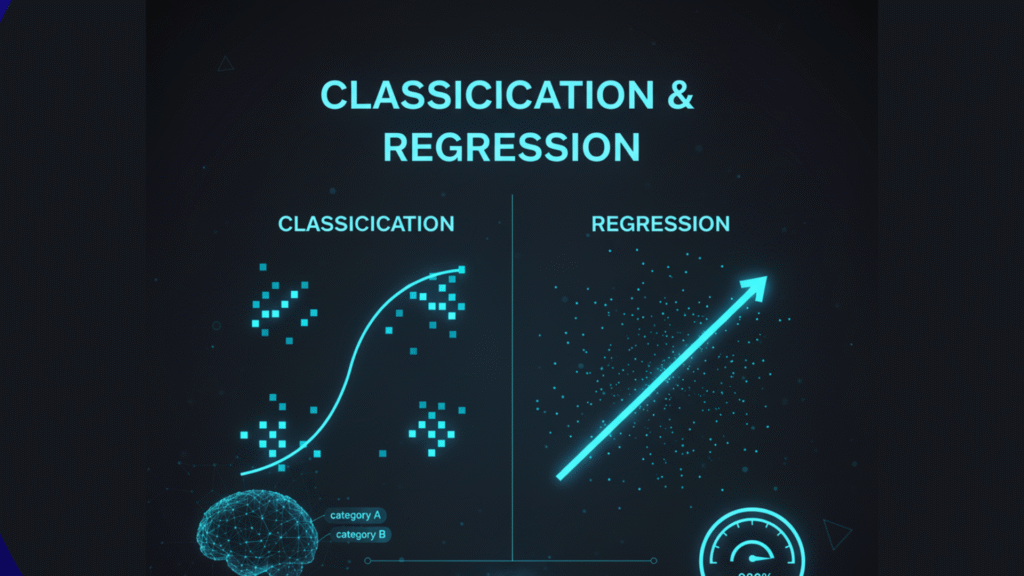
Supervised Learning problems are broadly categorized into two main types, distinguished by the nature of the output variable Y. Understanding this distinction is the first critical step in applying Supervised Learning correctly.

1. Classification: Predicting Discrete Categories

When the output variable is a category or a class, we are dealing with a classification problem. The algorithm is tasked with placing the input data into one of several discrete, pre-defined buckets. The output is essentially a label.

Real-World Examples of Classification in Supervised Learning:

• Email Spam Detection: Input: email text, metadata; Output: “Spam” or “Not Spam” (a binary classification).
• Medical Diagnosis: Input: patient symptoms, lab results, medical images; Output: “Disease Present” or “Disease Absent,” or even specific disease types (multi-class).
• Image Recognition: Input: image pixels; Output: “Cat”, “Dog”, “Car”, “Pedestrian”, etc. This is a classic application of Supervised Learning in computer vision.
• Sentiment Analysis: Input: tweet or product review text; Output: “Positive”, “Negative”, or “Neutral”. This uses Supervised Learning for natural language processing.
• Loan Approval: Input: applicant’s income, credit score, age; Output: “Approve” or “Deny”.

Classification can be binary (two classes) or multi-class (more than two classes). The core mechanics of the Supervised Learning algorithm adjust based on this, but the fundamental goal remains the same: assign a category.

2. Regression: Predicting Continuous Values

When the output variable is a real, continuous value (a number), we are dealing with a regression problem. Here, the algorithm is tasked with predicting a quantity on a continuous scale.

Real-World Examples of Regression in Supervised Learning:

• House Price Prediction: Input: square footage, number of bedrooms, location, school district quality; Output: Price (e.g., $450,000). This is a quintessential regression problem.
• Stock Market Forecasting: Input: historical prices, trading volume, news sentiment, economic indicators; Output: Future stock price at a specific time.
• Weather Prediction: Input: atmospheric pressure, humidity, wind speed, historical trends; Output: Temperature, rainfall amount.
• Sales Forecasting: Input: historical sales data, marketing spend, seasonality, competitor pricing; Output: Next quarter’s sales revenue.
• Drug Response Prediction: Input: patient genomics, dosage; Output: Reduction in symptom severity on a continuous scale.

The key distinction is simple but profound: Classification predicts a label, Regression predicts a quantity. Choosing the correct type is the first and most critical decision in setting up a Supervised Learning task.

The Supervised Learning Workflow: A Step-by-Step Guide for Practitioners

Building a robust Supervised Learning model is a systematic and iterative process. It’s more of a craft than a simple recipe. Here’s a detailed breakdown of the typical pipeline a data scientist follows in a Supervised Learning project.

Step 1: Data Collection and Problem Formulation
This is the foundational step. Before a single line of code is written, the business problem must be clearly defined. What are we trying to predict? Once defined, you need a sufficient volume of high-quality, labeled data. The source could be SQL databases, APIs, web scraping, or public datasets. The axiom “garbage in, garbage out” is never truer than in Supervised Learning.

Step 2: Data Preprocessing and Exploratory Data Analysis (EDA)
Raw data is almost never ready for modeling. This stage, often the most time-consuming part of a Supervised Learning project, involves:

• Handling Missing Values: Deciding whether to remove rows with missing data or impute (fill in) them using methods like mean/median/mode imputation or more advanced techniques like k-Nearest Neighbors imputation.
• Categorical Encoding: Converting non-numerical categories (e.g., “Red,” “Blue”, “Paris”, “London”) into numerical representations that algorithms can understand. Techniques include One-Hot Encoding (creating binary columns) or Label Encoding (assigning an integer).
• Feature Scaling: Standardizing or normalizing numerical features to bring them onto a similar scale. This is crucial for algorithms like Support Vector Machines and K-Nearest Neighbors that are sensitive to the magnitude of data. Methods include StandardScaler (zero mean, unit variance) and MinMaxScaler (scaling to a range like [0,1]).
• Exploratory Data Analysis (EDA): Using visualizations (histograms, box plots, scatter plots, correlation matrices) and statistical summaries to understand the data’s distribution, identify outliers, detect multicollinearity, and uncover initial relationships between variables. EDA guides the entire Supervised Learning process.

Step 3: Data Splitting: The Foundation of Generalization
We strategically split the labeled dataset into (at least) two distinct parts to rigorously evaluate our Supervised Learning model:

• Training Set: The bulk of the data (typically 70-80%) used to train the model. This is the “textbook” the student learns from. The model’s parameters are adjusted based solely on this data.
• Test Set: The remaining data (20-30%) is held back and used only once to evaluate the final model’s performance. This is the “final exam” that tests how well the student can generalize to completely new information. Data leakage from the test set into the training process fatally compromises the evaluation.

A common best practice is to also create a Validation Set from the training data (e.g., using a 60/20/20 split) to tune the model’s hyperparameters during development, ensuring the final test set remains a pure, unbiased measure of generalization.

Step 4: Model Selection
This is where we choose the appropriate algorithm for our Supervised Learning task. The choice depends on the problem type (classification or regression), the size and nature of the data, the desired level of interpretability, and computational constraints. We’ll explore specific algorithms in the next section.

Step 5: Model Training: The Core of Learning
The chosen algorithm is “fit” to the training data. Mathematically, this is an optimization process where the model’s internal parameters are adjusted to minimize the difference between its predictions and the actual labels in the training set. This difference is quantified by a loss function (or cost function), such as Cross-Entropy for classification or Mean Squared Error for regression. The optimizer (like Gradient Descent) navigates this loss landscape to find the optimal parameters.

Step 6: Model Evaluation and Interpretation
We use the untouched test set to assess the model’s performance. We feed the test inputs to the model, get its predictions, and compare them to the true test labels.

• For Classification: Common metrics include Accuracy, Precision, Recall, F1-Score, and the Confusion Matrix. The choice of metric is business-dependent.
• For Regression: Common metrics include Mean Absolute Error (MAE), Mean Squared Error (MSE), Root Mean Squared Error (RMSE), and R-squared (R²).

Furthermore, we use techniques like SHAP and LIME to interpret complex models, understanding which features drove specific predictions.

Step 7: Hyperparameter Tuning and Optimization
Models have hyperparameters—configuration settings that are not learned from the data but are set prior to training (e.g., the depth of a Decision Tree, the learning rate of a neural network). Using the validation set, we search for the best combination of these hyperparameters to optimize performance. Techniques like Grid Search (exhaustive search), Random Search (random sampling), and more advanced methods like Bayesian Optimization are commonly used in sophisticated Supervised Learning pipelines.

Step 8: Prediction, Deployment, and Monitoring
Once satisfied with the model’s performance on the test set, it’s ready for the real world. It can be deployed as part of an application, website, or system to make predictions on new, unlabeled data. However, the job isn’t done. Models in production can suffer from “model drift” where performance degrades over time as the underlying data distribution changes, requiring continuous monitoring and potential retraining—a key aspect of maintaining a Supervised Learning system in production.

A Tour of Essential Supervised Learning Algorithms

The field of Supervised Learning offers a diverse and powerful toolkit. Let’s meet the key “students” in our machine learning classroom, from simple classics to complex powerhouses.

Linear Models: The Simple Yet Powerful Workhorses

• Linear Regression: The go-to algorithm for regression tasks. It assumes a linear relationship between the input features X and the continuous output Y. It fits a straight line (or a hyperplane in higher dimensions) to the data by finding the coefficients that minimize the sum of squared errors. Its simplicity, speed, and interpretability make it a vital baseline model in any Supervised Learning regression task.
• Logistic Regression: Despite its name, it’s a fundamental classification algorithm. It models the probability that an input belongs to a particular class using a logistic function (sigmoid). It’s excellent for binary classification and provides probabilistic interpretations, which is incredibly valuable for decision-making under uncertainty.

Tree-Based Models: Mimicking Human Decision-Making

• Decision Trees: These models learn a hierarchy of simple, human-readable decision rules inferred from the data features, creating a tree-like structure. They are highly interpretable—you can literally trace the path of a decision. For example: “If Age > 30 and Credit Score > 650, then Approve Loan.” However, they are prone to overfitting.
• Random Forest: An ensemble method that builds a “forest” of many decision trees and combines their results (e.g., through majority voting for classification). It’s like asking a diverse committee of experts for their opinion. This “wisdom of the crowd” approach, where each tree is trained on a random subset of data and features, significantly reduces overfitting and is often one of the most accurate and robust algorithms for Supervised Learning.
• Gradient Boosting Machines (e.g., XGBoost, LightGBM, CatBoost): Another powerful ensemble technique. Instead of building trees in parallel (like Random Forest), it builds them sequentially, where each new tree is trained to correct the errors (residuals) of the previous one. This focused, iterative correction makes Gradient Boosting extremely powerful and often the winner of machine learning competitions. XGBoost, in particular, is a champion algorithm for structured/tabular data.

Distance-Based and Probabilistic Models

• K-Nearest Neighbors (KNN): A simple, instance-based, and non-parametric algorithm. To classify a new data point, it looks at the ‘K’ data points in the training set that are closest to it (in feature space) and assigns the most common class among them. For regression, it takes the average value. Its performance heavily relies on good feature scaling and distance metrics.
• Naïve Bayes: A family of probabilistic classifiers based on applying Bayes’ theorem with strong (naïve) independence assumptions between the features. They are remarkably fast, work well with high-dimensional data (like text), and are a popular choice for text classification and spam filtering within Supervised Learning applications.

Advanced and Flexible Models

• Support Vector Machines (SVM): A powerful classifier that finds the optimal “hyperplane” that best separates the classes in the feature space, aiming for the widest possible margin. It can handle non-linear relationships using the “kernel trick,” which implicitly maps data to a higher-dimensional space. SVMs are effective in high-dimensional spaces and are memory efficient.
• Neural Networks: Inspired by the human brain, these are highly flexible models composed of interconnected layers of nodes (neurons). They are capable of learning extremely complex, non-linear relationships and hierarchical features. They are the foundation of deep learning and excel with very large, high-dimensional data like images (Convolutional Neural Networks), text (Recurrent Neural Networks, Transformers), and audio. While often seen as “black boxes,” they represent the cutting edge of Supervised Learning for complex pattern recognition.

Evaluating Model Performance: Beyond Simple Accuracy

Judging a Supervised Learning model isn’t just about how often it’s right. The choice of the right metric is dictated by the business context and the consequences of different types of errors.

Key Metrics for Classification:

• Accuracy: (Correct Predictions / Total Predictions). A good general measure but can be dangerously misleading for imbalanced datasets (e.g., if 99% of transactions are not fraudulent, a model that always predicts “not fraud” will be 99% accurate but useless).
• Confusion Matrix: A fundamental table that breaks down predictions into four crucial categories, providing a complete picture of model performance:
  • True Positives (TP): Correctly predicted positive classes.
  • True Negatives (TN): Correctly predicted negative classes.
  • False Positives (FP): Incorrectly predicted positive (Type I error).
  • False Negatives (FN): Incorrectly predicted negative (Type II error).
• Precision: (TP / (TP + FP)). Answers: “Of all the instances we predicted as positive, how many are actually positive?” Crucial when the cost of FP is high (e.g., in spam detection, you don’t want good emails marked as spam; in targeted marketing, you want a precise audience).
• Recall (Sensitivity): (TP / (TP + FN)). Answers: “Of all the actual positive instances, how many did we correctly predict?” Crucial when the cost of FN is high (e.g., in cancer screening, you don’t want to miss any sick patients; in fraud detection, you want to catch as many fraudulent transactions as possible).
• F1-Score: The harmonic mean of Precision and Recall. A single metric that balances both concerns, useful when you need to find a compromise between the two.
• ROC Curve & AUC: The Receiver Operating Characteristic curve plots the True Positive Rate (Recall) against the False Positive Rate at various classification thresholds. The Area Under the Curve (AUC) provides a single measure of overall model performance across all thresholds, with 1.0 being a perfect model and 0.5 being no better than random guessing.

Key Metrics for Regression:

• Mean Absolute Error (MAE): The average of the absolute differences between predictions and actual values. It is robust to outliers and easy to interpret (e.g., “our house price predictions are off by $10,000 on average”).
• Mean Squared Error (MSE): The average of the squared differences. It penalizes larger errors much more heavily than MAE. Its square root, RMSE, is useful as it is in the same units as the original output variable.
• R-squared (R²): Represents the proportion of the variance in the dependent variable that is predictable from the independent variables. It’s a measure of how well the model fits the data compared to a simple mean model, with 1 being a perfect fit and 0 indicating the model explains none of the variance.

The Crucial Balancing Act: Bias vs. Variance & The Perils of Overfitting

This is one of the most fundamental concepts in machine learning and a central challenge in any Supervised Learning project. The bias-variance tradeoff is a key concept for understanding model performance in Supervised Learning.

• Bias: Error due to overly simplistic assumptions in the model. A high-bias model is underfit—it fails to capture the underlying trends in the data. It is often too simple. Both training and test error are high. Think of it as a student who only read the summary of the textbook and cannot answer detailed questions.
• Variance: Error due to excessive complexity in the model. A high-variance model is overfit—it learns the training data, including its noise and random fluctuations, too well. It performs excellently on the training data but poorly on the test data because it has effectively “memorized” the training set instead of learning the generalizable pattern. Think of a student who memorized the textbook word-for-word but cannot apply the concepts to new, slightly different questions.

The goal of every Supervised Learning practitioner is to find the sweet spot that balances bias and variance, leading to a model that is complex enough to capture the true patterns but simple enough to generalize well to new data.

Techniques to Combat Overfitting in Supervised Learning:

• Cross-Validation: A robust resampling technique (like k-fold CV) for assessing generalizability by repeatedly splitting the training data into different folds for training and validation. It provides a more reliable estimate of model performance than a single train-validation split.
• Regularization (L1 Lasso & L2 Ridge): A technique that adds a penalty for model complexity (the magnitude of coefficients) to the loss function. This discourages the model from becoming too complex and relying too heavily on any single feature, effectively simplifying it and reducing variance.
• Pruning: For Decision Trees, cutting back the tree after it has been built by removing branches that have little power in predicting the target variable, thereby reducing its complexity.
• Using Ensemble Methods: Like Random Forest and Gradient Boosting, which naturally reduce variance by combining multiple models.
• Early Stopping: For iterative algorithms like neural networks and boosting, stopping the training process before the model has fully converged on the training data, preventing it from learning the noise.

Challenges, Limitations, and Ethical Considerations in Supervised Learning

Despite its immense power, Supervised Learning is not a magic bullet. A responsible data scientist must be aware of its inherent challenges and limitations, which are critical considerations in any Supervised Learning project.

1. Dependency on Vast Amounts of Labeled Data: Acquiring large, high-quality, accurately labeled datasets is often the single biggest bottleneck. It is expensive, time-consuming, and requires significant expert knowledge (e.g., radiologists to label medical images).
2. Human Bias in Data: This is a critical issue of fairness and ethics in AI. If the historical data used to train the model contains human or societal biases (e.g., biased hiring data, prejudiced judicial records), the model will learn, perpetuate, and often amplify these biases. A Supervised Learning model is not objective; it reflects the data it was trained on. Techniques for debiasing data and models are an active area of research.
3. Limited to Known Classes/Outputs: A classification model can only predict classes it has seen during training. It cannot handle novel, unseen categories (the “open world” problem). Similarly, a regression model may perform poorly if asked to extrapolate far beyond the range of its training data.
4. The Black Box Problem: Complex models like deep neural networks and large ensemble methods can be incredibly accurate but are often difficult or impossible to interpret. Understanding why a model made a particular decision is crucial for building trust, meeting regulatory requirements (like GDPR’s “right to explanation”), and debugging. The field of Explainable AI (XAI) is dedicated to solving this.
5. Feature Engineering Dependency: The performance of many Supervised Learning algorithms is heavily dependent on the quality of the input features. Extracting, selecting, and creating informative features (feature engineering) remains a key skill, though deep learning has automated some of this for unstructured data.

Conclusion: The Indispensable Tool in the Data Scientist’s Toolkit

In conclusion, Supervised Learning is the bedrock upon which much of predictive analytics and modern AI is built. From the simple, interpretable elegance of a linear regression to the formidable, complex power of a gradient-boosted forest or a deep neural network, it provides a rich and diverse toolkit for solving a vast array of real-world problems. Mastering the concepts of Supervised Learning—from the foundational workflow and the array of algorithms to the nuanced evaluation metrics and the critical bias-variance trade-off—is non-negotiable for any aspiring data scientist or machine learning engineer. It is a field that beautifully blends statistics, computer science, and domain expertise to create systems that can learn from the past to predict the future.

As you move forward in your data science journey, remember that building a great Supervised Learning model is as much an art as it is a science. It requires careful data preparation, thoughtful algorithm selection, rigorous evaluation, and a deep sense of ethical responsibility. Now that you’re armed with this comprehensive knowledge, you are well-prepared to start your own Supervised Learning projects, contribute to the intelligent systems of tomorrow, and continue exploring the ever-evolving landscape of machine learning. The journey into Supervised Learning is a continuous learning process, but it is one of the most rewarding paths in technology today.