5 Powerful Activation Functions Every Data Scientist Should Know in 2025

In the intricate architecture of a neural network, the Activation Function is not merely a component; it is the very soul that introduces non-linearity and enables the network to learn complex patterns from data. Without it, a neural network, regardless of its depth, would be nothing more than a simple linear regression model. As we advance into 2025, the choice of Activation Function remains a critical hyperparameter that can dramatically influence training dynamics, convergence speed, and ultimate model performance. This article delves into five powerful Activation Functions that every data scientist must master, moving beyond the classic ReLU to explore modern, adaptive functions that are shaping the state-of-the-art in deep learning.

The Fundamental Role of an Activation Function

Before we explore specific functions, it’s crucial to understand their universal purpose. An Activation Function is a mathematical gate that is applied to the output of a neuron. It determines whether and to what extent a signal should progress through the network.

The two primary roles of an Activation Function are:

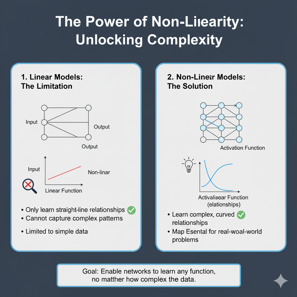
1. Introducing Non-Linearity: Real-world data is inherently non-linear. Functions like y = mx + c are insufficient to model complex phenomena like image recognition, natural language processing, or financial forecasting. By applying a non-linear Activation Function, we allow the network to create complex, non-linear mappings between inputs and outputs, making it a universal function approximator.
2. Controlling the Output Range: Different Activation Functions constrain the output to a specific range (e.g., 0 to 1, -1 to 1). This is vital for stability in training, especially in the output layer. For instance, a sigmoid function is ideal for binary classification as it squashes outputs into a probability between 0 and 1.

The journey of activation functions is one of evolution, driven by the need to solve specific problems like the “vanishing gradient” problem. Let’s begin with the function that started a revolution.

How Activation Functions Solve This:
By applying a non-linear function (like ReLU, Sigmoid, etc.) to the linear output z, we break the linearity. The neuron’s output becomes a = f(z), where f is non-linear.

When you stack multiple layers of these non-linearly activated neurons, each layer performs a non-linear transformation on the output of the previous layer. This creates a composite function of immense complexity. This is the “universal approximation theorem” in action: a neural network with even a single hidden layer and a non-linear activation function can theoretically approximate any continuous function, given enough neurons.

Analogy: Think of building with LEGO. Linear transformations are like having only straight bricks. You could only build walls. Non-linear activations are like adding curved bricks, hinges, and gears. Suddenly, you can build cars, castles, and robots.

2. Controlling the Output Range

What it Means:
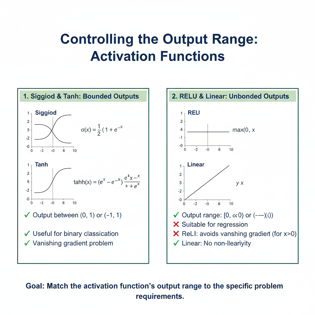
Different activation functions map the input (the weighted sum z) to different output ranges. This is crucial for both numerical stability and interpreting the network’s final output.

Why This is Important:

1. Preventing Numerical Explosion: Without a bounding function, the outputs of successive layers could grow exponentially large (a problem known as “activation explosion”), making training unstable and causing numerical overflow.
2. Suitable Outputs for the Task:
   • Binary Classification: The output needs to be a probability between 0 and 1. The Sigmoid function is perfect for this, as its range is (0, 1).
   • Multi-class Classification: The outputs should be probabilities that sum to 1. The Softmax function (a multi-dimensional generalization of Sigmoid) is used here.
   • Regression with no bounds: For predicting a value like a house price, you might use a linear activation (no activation) in the output layer, as its range is (-∞, +∞).
   • Regression with positive values: For predicting something like age or a pixel intensity, ReLU can be useful as it ensures the output is never negative.
3. Gradient Dynamics: The output range directly influences the size of the gradients during backpropagation. A function with a small output range (like Tanh between -1 and 1) tends to produce smaller gradients, which can contribute to the “vanishing gradient” problem if not managed carefully.

2. The Five Essential Activation Functions

2.1 ReLU (Rectified Linear Unit)

Detailed Mechanics:
f(x) = max(0, x)

• If the input x is positive, the output is x.
• If the input x is negative or zero, the output is 0.

In-Depth Analysis of “Why it’s Powerful”:

• Sparsity: When a ReLU neuron outputs zero, it is effectively “inactive.” In a large network, this means that for any given input, only a subset of neurons are active. This is beneficial because:
  • Efficiency: Sparse representations are computationally cheaper to process.
  • Representation Power: It forces the network to learn specialized, non-redundant features. Different inputs activate different pathways through the network, much like different thoughts activate different pathways in the human brain.
• Mitigates Vanishing Gradient: Compare ReLU to the old Sigmoid function. The derivative of Sigmoid is sigmoid(x)*(1-sigmoid(x)), which has a maximum value of 0.25. When you multiply these small gradients together across many layers during backpropagation, the gradient can become vanishingly small. ReLU’s derivative for positive inputs is exactly 1. This constant, strong gradient signal flows backwards largely unimpeded, allowing deep networks to learn effectively. This was a breakthrough that enabled the training of very deep networks.
• Computational Efficiency: It involves a simple comparison and a pass-through—operations that are trivial for a CPU or GPU to compute. This is far faster than computing exponentials (as in Sigmoid/Tanh) or logarithms.

The “Dying ReLU” Problem – A Deep Dive:

This is ReLU’s critical flaw. Let’s trace how a neuron dies:

1. A large gradient update or an unfortunate weight initialization causes a neuron’s weights to become such that for all data points in the training set, the weighted sum z is negative.
2. The neuron’s output becomes 0 for every input.
3. During backpropagation, the gradient of ReLU for a negative input is 0.
4. Therefore, the gradient for all weights leading into this neuron will be 0.
5. If the gradient is zero, the weights will not update. The neuron is permanently dead—it contributes nothing to the network’s learning and will never recover.

This is especially problematic with high learning rates, which can cause large, damaging weight updates.

2.2 Leaky ReLU & PReLU – The Evolved ReLU

Detailed Mechanics:

• Leaky ReLU: f(x) = max(αx, x). Here, α is a small, fixed constant (typically 0.01). It’s a “leak” that allows a tiny, non-zero gradient when the unit is not active.
• Parametric ReLU (PReLU): f(x) = max(αx, x). The key difference is that α is a learnable parameter. It starts with an initial value (often 0.25) and is updated via gradient descent along with the other weights of the network.

In-Depth Analysis of “Why they’re Powerful”:

• Prevents Neuron Death: By having a small, negative slope (α), Leaky ReLU ensures that even if a neuron’s pre-activation is negative, it still has a non-zero output and, crucially, a non-zero gradient. This gradient, however small, allows the weights to potentially recover and become active again in the future. It solves the “Dying ReLU” problem.
• PReLU – The Learnable Leak: Leaky ReLU’s α is a hyperparameter. Who’s to say 0.01 is the best value for all layers and all datasets? PReLU answers this by letting the network decide.
  • The network can learn that for some layers, a more negative slope (a larger α) is beneficial, allowing more information from negative values to pass through.
  • For other layers, it might learn that a slope closer to zero (like standard ReLU) is better.
  • This adaptability often leads to better performance than a fixed leak, but it comes at the cost of adding one more parameter per neuron to learn, which increases model complexity and memory footprint slightly.

2.3 GELU (Gaussian Error Linear Unit)

Detailed Mechanics:
The GELU function is based on the idea of “stochastic regularization” like Dropout. Instead of randomly setting neurons to zero, GELU weights the input by its value. It asks: “How likely is it that this input would be ‘dropped out’?”

The exact formula involves the Gaussian cumulative distribution function (CDF), but the common approximation is:
GELU(x) ≈ 0.5x * (1 + tanh[√(2/π) * (x + 0.044715x³)])

In-Depth Analysis of “Why it’s Powerful”:

• Smooth & Non-Monotonic: Unlike ReLU’s hard, deterministic cut-off at zero, GELU has a smooth, curved transition. This smoothness is a desirable property in optimization, as it often leads to a more stable and well-behaved loss landscape, making it easier for gradient-based optimizers to find good minima. Its “non-monotonic” nature (it slightly dips for negative values before rising) is thought to allow for more nuanced transformations.
• Probabilistic Interpretation: This is its core innovation. GELU can be understood as:
  GELU(x) = x * P(X <= x) where X is a Gaussian variable.
  In simpler terms, the input x is scaled by the probability that it is “above” a stochastic threshold. A high, positive x has a high probability of being kept, so it’s largely unchanged. A value near zero has a ~50% chance, so it’s scaled down. This is a smoother, more data-aware form of gating than ReLU.
• Success in Transformers: The Transformer architecture, with its layer normalization and deep, complex interactions, seems to benefit greatly from GELU’s smooth, probabilistic nature. It has become an empirical standard, delivering more stable training and better final performance in models like BERT and GPT.

2.4 SwiGLU (Sigmoid-Weighted Linear Unit)

Detailed Mechanics:
SwiGLU is a specific variant of the Gated Linear Unit (GLU). A general GLU is:
GLU(x) = f(xW + b) ⊙ (xV + c)
where ⊙ is element-wise multiplication and f is a gating function (often sigmoid).

SwiGLU specifically uses the Swish function (x * sigmoid(βx)) as f:
SwiGLU(x) = (xW + b) * sigmoid(β(xV + c)) (often, β=1 and biases are omitted for simplicity).

In-Depth Analysis of “Why it’s Powerful”:

• Gating Mechanism: The magic is in the element-wise multiplication (⊙). The left side (xW + b) is the “value” or “candidate activation.” The right side sigmoid(xV + c) is the “gate.” This gate outputs a value between 0 and 1 for each neuron.
  • A gate value of 1 means “let all information through.”
  • A gate value of 0 means “block all information.”
  • A value of 0.7 means “let 70% of the information through.”
    This allows the network to learn conditional computation. It can learn to open pathways for some types of inputs and close them for others, creating much more expressive and powerful transformations than a simple non-linearity.
• The Power of Swish: The Swish gate is superior to a raw sigmoid gate because it is smooth and non-monotonic. It doesn’t have a hard saturation point, which helps mitigate the vanishing gradient problem within the gating mechanism itself. Research has shown that Swish generally works better than sigmoid in this context.
• Empirical Superiority: The 2020 paper “GLU Variants Improve Transformer” tested this extensively. SwiGLU consistently outperformed the standard GELU-activated feed-forward network in Transformers. The added computational cost of the gating mechanism is justified by the significant boost in model quality and data efficiency.

2.5 Mish

Detailed Mechanics:
Mish(x) = x * tanh(softplus(x)) where softplus(x) = ln(1 + e^x).

Let’s break this down:

1. softplus(x) is a smooth, differentiable approximation of ReLU.
2. tanh(softplus(x)) takes this smoothed ReLU and squashes it to the range (0, 1), but in a smooth, graded way.
3. Multiplying by x gives the final output.

In-Depth Analysis of “Why it’s Powerful”:

• Smooth and Non-Monotonic: Like GELU and Swish, Mish avoids sharp corners and hard zero boundaries. Its smoothness creates a very “well-behaved” loss landscape, which allows gradient descent to traverse it more effectively and find better minima. The small allowance for negative values (it asymptotically approaches 0 as x -> -∞, but never quite reaches it) helps preserve information.
• Self-Regularization: The author of Mish argues that its shape naturally prevents overfitting. The idea is that the function’s ability to allow small negative values acts as a regularizer by maintaining a more diverse set of activations, preventing the network from becoming over-confident on specific features. In practice, users often find they can use less explicit regularization (like dropout) when using Mish.
• Performance in Vision Tasks: In rigorous benchmarks across ImageNet, CIFAR, and object detection tasks, Mish has been shown to provide a consistent, albeit sometimes small, accuracy gain over ReLU and often outperforms other modern activations. It seems particularly well-suited to the hierarchical feature learning that occurs in CNNs. The trade-off is its higher computational cost due to the tanh and softplus operations.

3. A Practical Guide for 2025: How to Choose and Implement

Understanding the theory is one thing; knowing how to apply it in practice is another. This section provides a concrete decision framework and implementation details for using these activation functions effectively in your 2025 projects.

3.1 The Activation Function Decision Framework

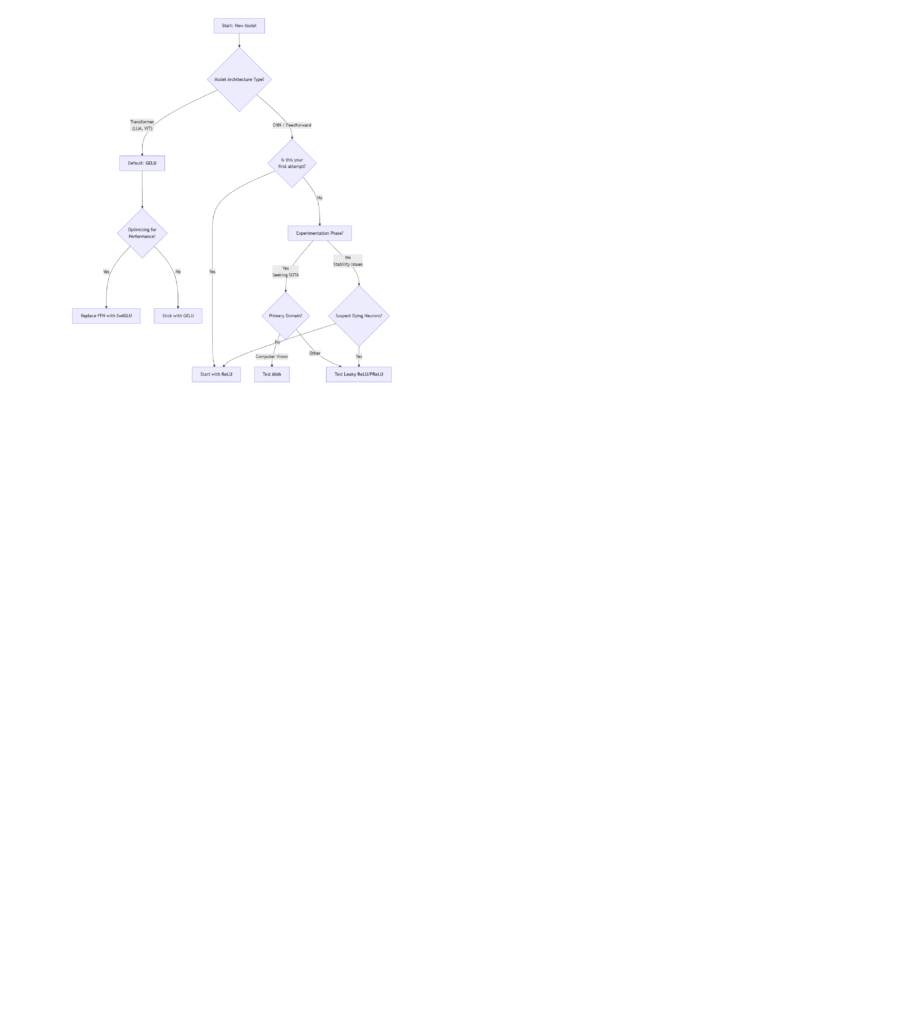
Choosing the right Activation Function is rarely a one-size-fits-all process, but this flowchart provides a robust starting point for any project in 2025:

Step-by-Step Guide to the Framework:

1. Identify Your Architecture:
   • Transformer-based Models (BERT, GPT, ViT): Your default choice is GELU. It is deeply integrated into these architectures and has been proven to work best with layer normalization and the attention mechanism. It is the safe, standard, and high-performing choice.
   • CNNs and Standard Feedforward Networks: This is where you have more flexibility. Begin with Step 2.
2. For CNNs/Feedforward Networks: Establish Your Baseline
   • First Pass / Default Baseline: Always start with ReLU. It is fast, simple, and works surprisingly well for a vast number of problems. Establish your model’s performance with ReLU first; this gives you a benchmark against which to measure more complex functions.
   • If You Suspect “Dying ReLU”: If your model’s loss gets stuck, learning is slow, or you notice a large proportion of zero activations in your network, switch to Leaky ReLU or PReLU. They are almost drop-in replacements that solve this specific problem.
3. The Experimentation Phase (Pushing for State-of-the-Art)
   Once you have a baseline, you can experiment to squeeze out extra performance.
   • For Computer Vision Tasks (Image Classification, Object Detection): Mish is your prime candidate. Its self-regularizing properties and smooth loss landscape have consistently shown superior results on benchmarks like ImageNet and COCO. Be prepared for a slight increase in computation time.
   • For Other Tasks / General Purpose: Leaky ReLU and PReLU are excellent general-purpose upgrades over ReLU. If you don’t want to add the complexity of a learnable parameter, use Leaky ReLU (α=0.01). If you have a larger model and the compute budget to tune more parameters, PReLU often yields a small but consistent performance improvement.
   • Optimizing Transformer Feed-Forward Networks: If you are designing or modifying a Transformer architecture and are seeking maximum performance, replace the standard Linear -> GELU -> Linear feed-forward block with a SwiGLU variant. This is a structural change, not just a layer swap, but it is currently the state-of-the-art for this component.

3.2 Implementation Code Snippets (2025 Standards)

Here’s how to implement these functions in TensorFlow/Keras and PyTorch, including best practices.

TensorFlow/Keras:

python

import tensorflow as tf
from tensorflow.keras import layers, models, initializers
#Activation Function
# ReLU (Default) - You can use the `activation` arg directly.
model = models.Sequential([
    layers.Dense(128, activation='relu'),  # Simple ReLU
])

# Leaky ReLU - Created as a separate layer.
model.add(layers.Dense(128)) # No activation here first
model.add(layers.LeakyReLU(alpha=0.01)) # Then add LeakyReLU

# PReLU - 'alpha_initializer' can be used to set initial value.
model.add(layers.Dense(128))
model.add(layers.PReLU(alpha_initializer=initializers.Constant(0.25)))

# GELU - Available as a built-in string.
model.add(layers.Dense(128, activation='gelu'))

# Mish - Not built-in by default, but easy to define and use.
@tf.function
def mish(x):
    return x * tf.math.tanh(tf.math.softplus(x))
model.add(layers.Dense(128, activation=mish))

# SwiGLU - Requires a custom layer as it's more complex.
class SwiGLU(layers.Layer):
    def __init__(self, units, **kwargs):
        super().__init__(**kwargs)
        self.units = units
        self.dense = layers.Dense(units * 2) # Two parallel transformations

    def call(self, inputs):
        x = self.dense(inputs)
        x1, x2 = tf.split(x, 2, axis=-1) # Split into value and gate
        return x1 * tf.nn.silu(x2) # silu is Swish in TF
model.add(SwiGLU(units=128))

PyTorch:

python

import torch
import torch.nn as nn
import torch.nn.functional as F

# ReLU, Leaky ReLU, PReLU, GELU are in nn.Module
class MyModel(nn.Module):
    def __init__(self):
        super().__init__()
        self.linear = nn.Linear(784, 128)
        self.relu = nn.ReLU()
        self.leaky_relu = nn.LeakyReLU(0.01)
        self.prelu = nn.PReLU(num_parameters=128) # 'num_parameters' for learnable alphas
        # GELU is available
        self.gelu = nn.GELU()
        
        # Mish needs to be defined
        self.mish = nn.Mish() # Note: Mish is now standard in recent PyTorch versions (>=1.9)
        #Activation Function
    def forward(self, x):
        x = self.linear(x)
        x = self.mish(x) # Example usage
        return x
 #Activation Function
# SwiGLU in PyTorch
class SwiGLU(nn.Module):
    def __init__(self, in_features, hidden_features):
        super().__init__()
        self.w1 = nn.Linear(in_features, hidden_features, bias=False)
        self.w2 = nn.Linear(in_features, hidden_features, bias=False)
        self.v = nn.Linear(in_features, hidden_features, bias=False)
        
    def forward(self, x):
        # SwiGLU: (x @ w1) * silu(x @ w2)
        return F.silu(self.w1(x)) * self.w2(x)
        
# Example of using it in a Transformer block
class TransformerBlock(nn.Module):
    def __init__(self, dim, hidden_ratio=4):
        super().__init__()
        hidden_dim = int(dim * hidden_ratio)
        # Using SwiGLU as the Feed-Forward Network
        self.ffn = SwiGLU(in_features=dim, hidden_features=hidden_dim)
        # Output projection back to original dimension
        self.out_proj = nn.Linear(hidden_dim, dim)
        
    def forward(self, x):
        x = self.ffn(x)
        x = self.out_proj(x)
        return x

3.3 Key Considerations for 2025

• Computational Cost (FLOPs): ReLU < Leaky ReLU/PReLU ≈ GELU < Mish < SwiGLU. Always consider your inference latency and training budget. The performance gains of Mish and SwiGLU come with a real computational cost.
• Interaction with Normalization Layers: The choice of Activation Function interacts with normalization layers like Batch Norm and Layer Norm. The standard order is Linear/Conv -> Norm -> Activation. This has been extensively tested and is generally robust. GELU’s success in Transformers is closely tied to its use with Layer Normalization.
• Don’t Forget the Output Layer: The rules change for the output layer. Use:
  • Sigmoid for binary classification.
  • Softmax for multi-class classification.
  • Linear (or ReLU if outputs must be positive) for regression.

4. The Future of Activation Functions (2025 and Beyond)

The evolution of activation functions is not over. As architectures and hardware change, so too will our preferred non-linearities. Here are the key trends and areas of research that will define the next generation of activation functions.

4.1 The Shift from Deterministic to Adaptive & Smooth

The historical trend is clear:

1. Deterministic & Saturated: Sigmoid, Tanh (hard limits, vanishing gradients)
2. Deterministic & Non-Saturated: ReLU (simple, but has dying neuron problem)
3. Adaptive & Smooth: Leaky ReLU, PReLU, GELU, Swish, Mish (smooth curves, data-dependent behavior, better optimization landscapes)

The future belongs to the third category. The success of GELU and SwiGLU in state-of-the-art models proves that smooth, adaptive functions that can preserve information (even from negative inputs) are superior for optimizing very deep, complex networks.

4.2 Learnable and Meta-Learned Activation Functions

Why should we, the engineers, choose the activation function? What if the network could learn its own optimal non-linearity?

• PReLU was an early step in this direction, learning the slope of the negative part.
• Searchable Activation Spaces (NAS): Neural Architecture Search can be extended to search for the best activation function for different layers within a network. A search space might include ReLU, GELU, Swish, etc., and the NAS algorithm chooses the best one for each layer.
• Parametric Activation Functions: Functions like PAU (Parametric Activation Unit) propose a single, flexible mathematical form that can approximate many existing activations (Sigmoid, Tanh, ReLU, etc.) and learn new ones directly from data. The parameters of this function are learned during training.

4.3 Hardware-Aware Activation Function Design

As we push for faster inference on edge devices (phones, IoT sensors), the hardware implications of activation functions become critical.

• ReLU is king on current hardware because it maps to extremely simple and fast instructions.
• GELU and Mish, with their exponential and logarithmic operations, are more expensive.
• Future research will focus on designing activation functions that are both highly performant and hardware-friendly. This could involve:
  • Creating smooth, powerful functions that can be well-approximated by low-precision arithmetic (e.g., INT8).
  • Designing functions that are “friendlier” for emerging AI accelerator chips.

4.4 The Role of Explainable AI (XAI)

As we demand more from our models, not just in performance but also in interpretability, the role of the activation function in understanding what a network is learning will grow.

• Analyzing which neurons fire (i.e., have high activation values) for different inputs can be a form of introspection.
• Activation functions with gating mechanisms, like SwiGLU, inherently provide a form of explanation. The gate values tell you which parts of the information flow the model deemed important for a given input. Research into visualizing and interpreting these gates will be a key part of XAI.

5. Conclusion

The Activation Function is far from a solved problem or a mere implementation detail. It is a dynamic and crucial component that sits at the heart of a neural network’s ability to learn. The journey from the simple step of ReLU to the probabilistic gating of GELU and SwiGLU represents a significant evolution in our understanding of how to build effective learning systems.

For the data scientist in 2025, mastery of these tools is non-negotiable. The key takeaways are:

1. Move Beyond ReLU as a Default: While it’s a great starting point, understand its limitations. For new projects, especially with Transformers, GELU should be your new baseline.
2. Embrace Specialization: There is no single “best” function. SwiGLU dominates in Transformer feed-forward layers, Mish excels in computer vision, and PReLU solves specific stability issues in CNNs. Use the right tool for the job.
3. Think About the System: The choice of activation function is part of a larger system involving normalization layers, optimizer choice, and hardware constraints. Consider the whole picture.
4. Look to the Future: The trend is toward learnable, smooth, and hardware-aware functions. Staying abreast of this research will give you a competitive edge.

By deeply understanding and strategically applying these five powerful Activation Functions, you equip yourself to design more robust, accurate, and efficient neural networks, ready to tackle the complex challenges of the next generation of AI applications.