Master Dropout: A Complete Guide to Regularization in Deep Learning

Abstract

In the relentless pursuit of creating deep learning models that not only perform well on their training data but can also generalize effectively to unseen data, regularization stands as a cornerstone technique. Among the pantheon of regularization methods, Dropout emerges as one of the most elegant, influential, and widely adopted. Introduced over a decade ago, its simplicity and power have ensured its continued relevance in the era of billion-parameter transformers and diffusion models.

This comprehensive guide for 2025 delves deep into the world of Dropout, moving beyond a superficial understanding to explore its foundational principles, mathematical underpinnings, modern implementations, advanced variants, and its evolving role in contemporary architectures. We will demystify why randomly “dropping” neurons during training leads to more robust and powerful neural networks, making you a master of this essential regularization technique.

1. The Fundamental Problem: Overfitting in Deep Learning

Before we can appreciate the solution, we must first understand the problem it solves. Overfitting is the single greatest obstacle to building useful machine learning models.

1.1 What is Overfitting?

A model is said to be overfitted when it learns the training data too well—including its noise and random fluctuations—to the detriment of its performance on new, unseen data. Imagine a student who memorizes a textbook word-for-word but fails to understand the underlying concepts. When faced with exam questions phrased differently, they struggle. Similarly, an overfitted neural network has high variance and low bias; it becomes a complex “look-up table” for the training set rather than a generalizable function.

Visual Analogy: Think of fitting a curve to a set of data points. An underfitted model might be a straight line that misses the general trend. A well-fitted model would be a smooth curve that captures the essential pattern. An overfitted model would be a complex, wiggly curve that passes through every single data point perfectly but fails to predict new points accurately.

1.2 Why are Deep Neural Networks Prone to Overfitting?

Deep Neural Networks (DNNs) are particularly susceptible to overfitting due to several factors:

1. High Model Capacity: Modern DNNs often possess millions or even billions of parameters. This vast number of degrees of freedom allows them to model extremely complex, and sometimes spurious, relationships within the training data.
2. Limited and Noisy Data: In many real-world scenarios, the amount of high-quality, labeled training data is limited. When data is scarce, the model is more likely to latch onto idiosyncrasies.
3. Complex Feature Co-adaptations: During training, neurons can develop intricate dependencies on each other. A neuron might only be effective in the presence of a few other specific neurons. This “co-adaptation” makes the network fragile; if one pathway is disrupted during inference, the entire prediction can collapse.

This is where regularization comes in.

1.3 The Role of Regularization

Regularization is any modification we make to a learning algorithm that is intended to reduce its generalization error but not its training error. Its primary goal is to discourage the model from becoming overly complex and to encourage it to learn more robust and generalizable features.

Classical regularization techniques like L1 (Lasso) and L2 (Ridge) penalize large weights in the model by adding a term to the loss function. While effective, these methods have limitations in the context of deeply connected networks. This sets the stage for a more structural approach: Dropout.

2. Dropout Unveiled: The Core Concept

Dropout is a regularization technique for neural networks that addresses the problem of co-adaptation directly. First introduced in 2012 by Nitish Srivastava, Geoffrey Hinton, and others in their seminal paper “Dropout: A Simple Way to Prevent Neural Networks from Overfitting,” its idea is deceptively simple.

2.1 The Analogy: The Ensemble “Aha!” Moment

The best way to understand Dropout is through an analogy. Imagine you are preparing for a difficult exam. You could rely on a single, brilliant study partner. However, if that one person is sick on exam day, you’re in trouble. A much better strategy is to form a study group with multiple people. Each member of the group studies the material independently. During the exam, you average the answers from all members. This “ensemble” is far more robust; even if one member misunderstood a concept, the collective knowledge of the group will likely produce the correct answer.

Training a single, massive neural network is like relying on one brilliant study partner. It can memorize everything but might not be robust.

2.2 How Dropout Works: The Mechanism

Dropout operationalizes this ensemble idea within a single network during training.

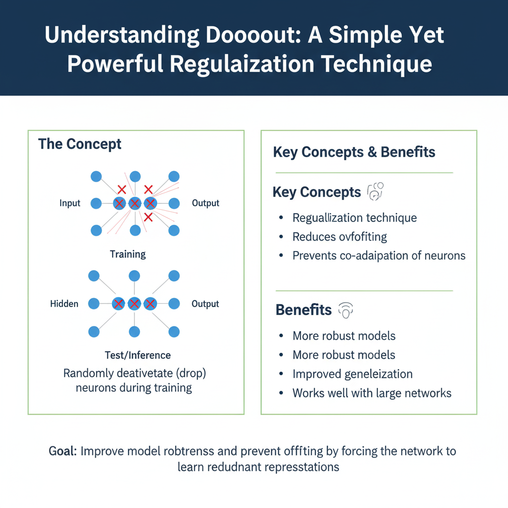
1. The Drop: For each training example, in every forward pass, Dropout randomly “drops out” (i.e., temporarily removes) a proportion of neurons in a layer. Each neuron is independently set to zero with a probability pp, known as the dropout rate. The connections to and from these dropped neurons are disabled for that single training step.
2. The Thinned Network: This results in a “thinned” network for that iteration. Since a different random set of neurons is dropped for every training example (or mini-batch), the network being trained is effectively a new, smaller architecture each time.
3. Preventing Co-adaptation: By randomly removing neurons, Dropout forces the network to avoid relying on any single neuron or any small set of neurons. It cannot count on specific connections being present. This breaks up co-adaptations, as neurons are forced to become more self-sufficient and to develop useful features on their own or in loose, redundant collaboration with others.
4. Inference (Testing): During testing or inference, Dropout is turned off. All neurons are active, but their outputs are scaled down by the dropout rate pp. This ensures that the expected output from a neuron at test time is the same as its expected output during training. Alternatively, a more common modern practice is Inverted Dropout, where the outputs of the remaining neurons are scaled up by 1/(1−p)1/(1−p) during training, leaving the network untouched during inference.

In essence, training with Dropout can be seen as training an exponential number of “thinned” subnetworks simultaneously that all share weights. At test time, you are effectively using a single, averaged ensemble of all these subnetworks.

3. The Mathematics and Intuition Behind Dropout

To move from a conceptual understanding to a practical implementation, we need to formalize the process mathematically.

3.1 The Forward Pass with Dropout

Let’s consider a single layer ll in a neural network with a vector of outputs y(l)y(l) that serves as the input to the next layer.

Without Dropout, the forward pass to the next layer is:z(l+1)=W(l+1)y(l)+b(l+1)z(l+1)=W(l+1)y(l)+b(l+1)y(l+1)=f(z(l+1))y(l+1)=f(z(l+1))

where ff is the activation function.

With Dropout applied to layer ll, we introduce a mask vector r(l)r(l). This vector is of the same dimension as y(l)y(l) and its elements are independent Bernoulli random variables with probability pp of being 0 (dropped) and 1−p1−p of being 1 (kept).

The forward pass becomes:y~(l)=r(l)⊙y(l)(Element-wise multiplication)y~​(l)=r(l)⊙y(l)(Element-wise multiplication)z(l+1)=W(l+1)y~(l)+b(l+1)z(l+1)=W(l+1)y~​(l)+b(l+1)y(l+1)=f(z(l+1))y(l+1)=f(z(l+1))

The key operation is the element-wise multiplication ⊙⊙, which zeroes out the activations of the dropped neurons.

3.2 The Scaling Problem: Why We Need Inverted Dropout

During training, the expected value of the output of a neuron is (1−p)⋅y(1−p)⋅y, because the neuron is only active (1−p)(1−p) fraction of the time. At test time, when all neurons are active, the expected input to the next layer would be yy. This mismatch in scale between training and testing would cause problems.

The original Dropout paper suggested solving this by scaling the weights at test time. However, the now-standard solution is Inverted Dropout, which performs the scaling during training.

In Inverted Dropout, we modify the forward pass:y~(l)=r(l)⊙y(l)1−py~​(l)=1−pr(l)⊙y(l)​

By dividing by (1−p)(1−p), we ensure that the expected value of y~(l)y~​(l) remains y(l)y(l) during training. This means that at test time, no scaling is necessary. The network can be run as-is with all neurons active, which is computationally efficient and simpler to implement. This is the method used in all modern deep learning frameworks.

3.3 Dropout as an Approximate Model Averaging

The original paper framed Dropout as an efficient way to perform model averaging with a vast number of neural networks. There are 2n2n possible “thinned” networks for a network with nn neurons. It’s intractable to train each of these networks separately and average their predictions.

Dropout provides a clever approximation:

1. Training: It trains all these 2n2n networks simultaneously by sharing their weights. Each training step updates the weights of one randomly sampled subnetwork.
2. Inference: The effect of averaging the predictions of all these subnetworks is approximated by using the full network with scaled weights (or, in the case of Inverted Dropout, by having already scaled the activations during training).

This Bayesian interpretation explains why Dropout networks are so robust: their predictions are effectively an average over a massive ensemble.

4. A Practical Guide to Implementing Dropout in 2025

Theory is essential, but implementation is where the rubber meets the road. Let’s explore how to use Dropout effectively with modern frameworks and best practices.

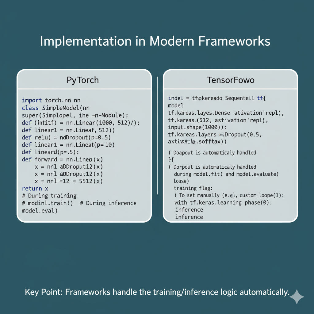
4.1 Implementation in Modern Frameworks

Implementing Dropout is trivial in frameworks like TensorFlow/Keras and PyTorch, as it’s available as a standard layer.

In TensorFlow/Keras:

python

import tensorflow as tf
from tensorflow.keras import layers, models

model = models.Sequential()
model.add(layers.Dense(256, activation='relu', input_shape=(784,)))
model.add(layers.Dropout(0.5))  # 50% dropout rate
model.add(layers.Dense(128, activation='relu'))
model.add(layers.Dropout(0.3))  # 30% dropout rate
model.add(layers.Dense(10, activation='softmax'))

The Dropout layer is inserted after the layer whose outputs you want to drop. During training, it’s active; during model.evaluate() or model.predict(), it is automatically disabled.

In PyTorch:

python

import torch
import torch.nn as nn

class NeuralNetwork(nn.Module):
    def __init__(self):
        super().__init__()
        self.layer1 = nn.Linear(784, 256)
        self.layer2 = nn.Linear(256, 128)
        self.output = nn.Linear(128, 10)
        self.dropout1 = nn.Dropout(0.5)
        self.dropout2 = nn.Dropout(0.3)
        self.relu = nn.ReLU()

    def forward(self, x):
        x = self.relu(self.layer1(x))
        x = self.dropout1(x) # Apply dropout after activation
        x = self.relu(self.layer2(x))
        x = self.dropout2(x)
        x = self.output(x)
        return x

# During training, the model is in train mode:  is active.
model = NeuralNetwork()
model.train()

# During evaluation, switch to eval mode: is disabled.
model.eval()

In PyTorch, it’s crucial to set the model to .train() or .eval() mode to toggle Dropout and other layers like Batch Normalization on and off.

4.2 Hyperparameter Tuning: The Dropout Rate (p)

The dropout rate pp is the most important hyperparameter. It represents the probability of dropping a neuron.

• p=0p=0: No Dropout. The standard network.
• p=1p=1: All neurons are dropped; the network outputs nothing (useless).

Choosing the right rate is a balance:

• Too low (e.g., 0.1): The effect is negligible. The network may still overfit.
• Too high (e.g., 0.9): The network is starved of information and will fail to learn, leading to underfitting.

Best Practices and Rules of Thumb for 2025:

• Input Layer: A lower rate is common, typically 0.1 to 0.2. You don’t want to lose too much of your raw input data.
• Hidden Layers: A common starting point is 0.5. This is the “sweet spot” used in the original paper for fully connected layers. From there, you can tune it based on validation performance.
• Output Layer: It is generally not recommended to apply Dropout to the output layer, as it can make the output probabilities noisy and unstable.
• Wide vs. Narrow Layers: Wider layers (with more neurons) can often tolerate a higher  rate as there is more redundancy.
• Task-Dependent Tuning: For tasks with very small datasets, you might need a higher rate (e.g., 0.6-0.8) to combat severe overfitting. For larger datasets, a lower rate might suffice.

4.3 Where to Place Dropout Layers?

The conventional wisdom is to place the Dropout layer after the activation function (e.g., ReLU). The reasoning is that you are dropping the activated features. However, some research suggests placing it before the activation can also work. The standard practice and framework defaults (as seen in the code above) place it after.

Crucially, the interaction with Batch Normalization (BN) layers is important. BN is another key modern technique that standardizes the inputs to a layer. Using  and BN together can be tricky because the changing statistics due to can interfere with BN’s running estimates of mean and variance. The general recommendation is to place Dropout after the BN layer.

Recommended Order: Dense/Conv Layer -> Batch Norm -> Activation -> Dropout

5. Beyond Vanilla Dropout: Advanced Variants and Related Techniques

The core idea has inspired a family of more specialized and powerful variants.

5.1 Spatial Dropout for Convolutional Networks

Standard performs poorly on convolutional layers. Why? In convolutional layers, adjacent pixels in a feature map are highly correlated. Dropping a random neuron (pixel) does little to break co-adaptation, as the same information is often available in the neighboring pixels.

Spatial Dropout is the solution. Instead of dropping individual neurons, it drops entire feature maps. For a convolutional layer with a 3D output tensor of shape (height, width, channels), Spatial Dropout 1D drops entire 1D channels, and Spatial Dropout 2D (the most common) drops entire 2D feature maps (channels). This forces the network to learn redundant feature representations across channels.

Implementation:

python

# In Keras
model.add(layers.Conv2D(64, (3, 3), activation='relu'))
model.add(layers.SpatialDropout2D(0.3)) # Drops entire 2D feature maps

# In PyTorch, it's nn.2d for convolutional layers (check the docs for channel-wise behavior).

5.2 Variational Dropout for Bayesian Deep Learning

This variant is used in Recurrent Neural Networks (RNNs), particularly for sequence-to-sequence tasks. The key idea is to apply the same mask at every time step of the sequence, rather than a new random mask for each step. This is crucial for the RNN to maintain a consistent “memory” through time. Using different masks at each step would create excessive noise and prevent the RNN from learning long-range dependencies.

5.3 Monte Carlo (MC) Dropout: A Free Lunch for Uncertainty Estimation

One of the most exciting developments is MC , proposed by Yarin Gal as a theoretically grounded framework for uncertainty estimation in deep learning.

The core insight is that a network trained with  approximate Bayesian model. Therefore, instead of turning  off at test time, we can leave it on and perform multiple forward passes (e.g., 100 passes) for a single input. Each pass will yield a slightly different prediction due to the random dropping.

• The Mean of these predictions is the final prediction.
• The Variance of these predictions is a measure of the model’s uncertainty.

This is incredibly powerful for real-world applications:

• Safety-Critical AI: A self-driving car can be more cautious if its model shows high uncertainty about an object.
• Active Learning: The model can identify data points it is most uncertain about, so a human can label them.
• Out-of-Distribution Detection: The model will typically show high uncertainty for inputs that are very different from its training data.

python

# Pseudo-code for MC in PyTorch
model.eval() # But we keep active!
mc_predictions = []
for _ in range(100): # 100 stochastic forward passes
    pred = model(input_data)
    mc_predictions.append(pred)

mc_predictions = torch.stack(mc_predictions)
prediction_mean = mc_predictions.mean(dim=0)
prediction_uncertainty = mc_predictions.std(dim=0)

5.4 AlphaDropout and SELU

With the introduction of the Self-Normalizing (SELU) activation function, a specialized  variant called AlphaDropout was created. SELU networks have self-normalizing properties, meaning they naturally maintain a mean of 0 and standard deviation of 1. Standard Dropout disrupts this. AlphaDropout is designed to preserve the self-normalizing property by also adjusting the affine parameters of the activation function, ensuring the mean and variance remain stable.

6. Dropout in the Modern Deep Learning Landscape (2025 and Beyond)

The deep learning landscape has evolved significantly since 2012. With the rise of new architectures, is still relevant?

6.1 Dropout vs. Other Regularizers

• Weight Decay (L2): A classic and still very effective method. It acts as a direct constraint on the model’s weights.  is more structural. They are often used together.
• Batch Normalization (BN): While its primary purpose is to stabilize and accelerate training, BN also has a mild regularizing effect due to the noise introduced by mini-batch statistics. This has led some to believe that  is unnecessary when using BN. This is a misconception. While BN can reduce the need for , they are complementary and can be used together for even better performance, especially when a model is severely overfitting.
• Data Augmentation: The best form of regularization is more and varied data. Data augmentation artificially expands the training set and is arguably the most powerful regularization technique for tasks like image recognition. Data augmentation are almost always used in conjunction.
• Label Smoothing: This technique prevents the model from becoming overconfident in its predictions by “smoothing” the hard 0/1 labels. It’s particularly useful in combination with Dropout.

6.2 Dropout in Transformer and Attention-Based Models

The Transformer architecture, which powers LLMs like GPT-4 and vision models like ViT, uses a different kind of building block: the Attention mechanism.

• Attention Is All You Need (Original Paper): The original Transformer used in several key places:
  1. After the embedding layer.
  2. After the residual connection and layer normalization in each sub-layer (the “feed-forward” network within the Transformer block).
  3. On the attention weights themselves (though this is less common now).
• Modern Large Language Models (LLMs): In very large models trained on massive datasets, the role (often called resid_dropout or embd_dropout in these contexts) is more nuanced. Excessive  can hinder learning. Therefore, it’s common to see relatively low dropout rates (e.g., 0.1) or even its complete removal in the final stages of pre-training to maximize model capacity. However, it is still a critical tool for preventing overfitting during fine-tuning on smaller, specific datasets.

6.3 When Not to Use Dropout

Dropout is not a silver bullet. There are situations where it is less effective or even harmful:

1. Very Small Datasets: If your dataset is tiny, the noise might prevent any meaningful learning. In such cases, strong L2 regularization and extensive data augmentation might be preferable.
2. Recurrent Layers (without Variational ): As discussed, using standard Dropout in RNNs breaks their ability to model sequences. Use Variational  instead.
3. When Computational Overhead is a Concern: The training time is similar to without, but the network typically requires 2-3 times more epochs to converge because the training signal is noisier. If you are on an extremely tight compute budget, this might be a consideration.
4. In Certain Generative Models: Some architectures, like Normalizing Flows or certain types of Generative Adversarial Networks (GANs), have specific stability requirements that can be disrupted

7. Conclusion: Mastering Dropout as a Core Skill

From its elegant inception to its sophisticated modern variants,  has proven to be one of the most enduring and impactful ideas in deep learning. It is a technique that every practitioner must master.

Key Takeaways for 2025:

• Core Purpose: Dropout is a powerful, simple, and effective regularization technique that prevents overfitting by breaking complex co-adaptations between neurons.
• Mechanism: It works by randomly dropping neurons during training, forcing the network to learn robust, redundant features.
• Implementation: Use Inverted  (the framework default). Place Dropout layers after activation functions and be mindful of their interaction with Batch Normalization.
• Tuning: The dropout rate is critical. Start with 0.5 for hidden layers and tune from there. Use SpatialDropout for CNNs and Variational  for RNNs.
• Modern Relevance:  remains highly relevant, especially in Transformer architectures and for providing uncertainty estimates via MC .
• Holistic Strategy: is not a standalone solution. It is most effective when used as part of a holistic regularization strategy that includes Data Augmentation, Weight Decay, and Batch Normalization.

Mastering  is more than just knowing how to add a layer to your model. It’s about understanding the philosophy of robust learning, the intuition behind model ensembles, and the practical wisdom of when and how to inject structured noise to build AI systems that truly generalize. As we push the boundaries of AI in 2025 and beyond, this foundational knowledge will continue to be a cornerstone of effective model design.