Top 10 Neural Network Architectures Every Data Scientist Should Know

Introduction: The Architectural Revolution in Artificial Intelligence

The field of artificial intelligence is undergoing a renaissance, largely driven by advances in a technology inspired by the human brain: the Neural Network. At its core, a Neural Network is a computational model composed of interconnected layers of nodes, or “neurons,” that can learn to recognize patterns and relationships in data. While the concept dates back to the 1950s, it is the evolution of specific architectures—the blueprints that define how these layers are organized and connected—that has unlocked the modern era of deep learning.

Understanding these architectures is no longer a niche skill but a fundamental requirement for any data scientist. Just as a civil engineer must understand the differences between a suspension bridge and a cantilever bridge, a data scientist must understand the strengths, weaknesses, and optimal applications of various Neural Network designs. The choice of architecture directly dictates what kind of problems a model can solve, its efficiency, and its ultimate performance.

This article serves as a comprehensive guide to the top 10 Neural Network architectures that form the bedrock of modern AI. We will move from foundational networks that process simple tabular data to sophisticated designs that power breakthroughs in image recognition, language understanding, and creative generation.

For each architecture, we will delve into its fundamental principles, its inner workings, its quintessential applications, and provide a practical implementation blueprint. By mastering these blueprints, you will be equipped to select the right tool for any AI challenge and understand the forces shaping the technological landscape.

Part 1: The Foundational Feedforward Architectures

Before tackling complex data like images and sequences, we must start with the architectures designed to find patterns in structured, static data.

1. The Multilayer Perceptron (MLP): The Universal Approximator

Conceptual Foundation:
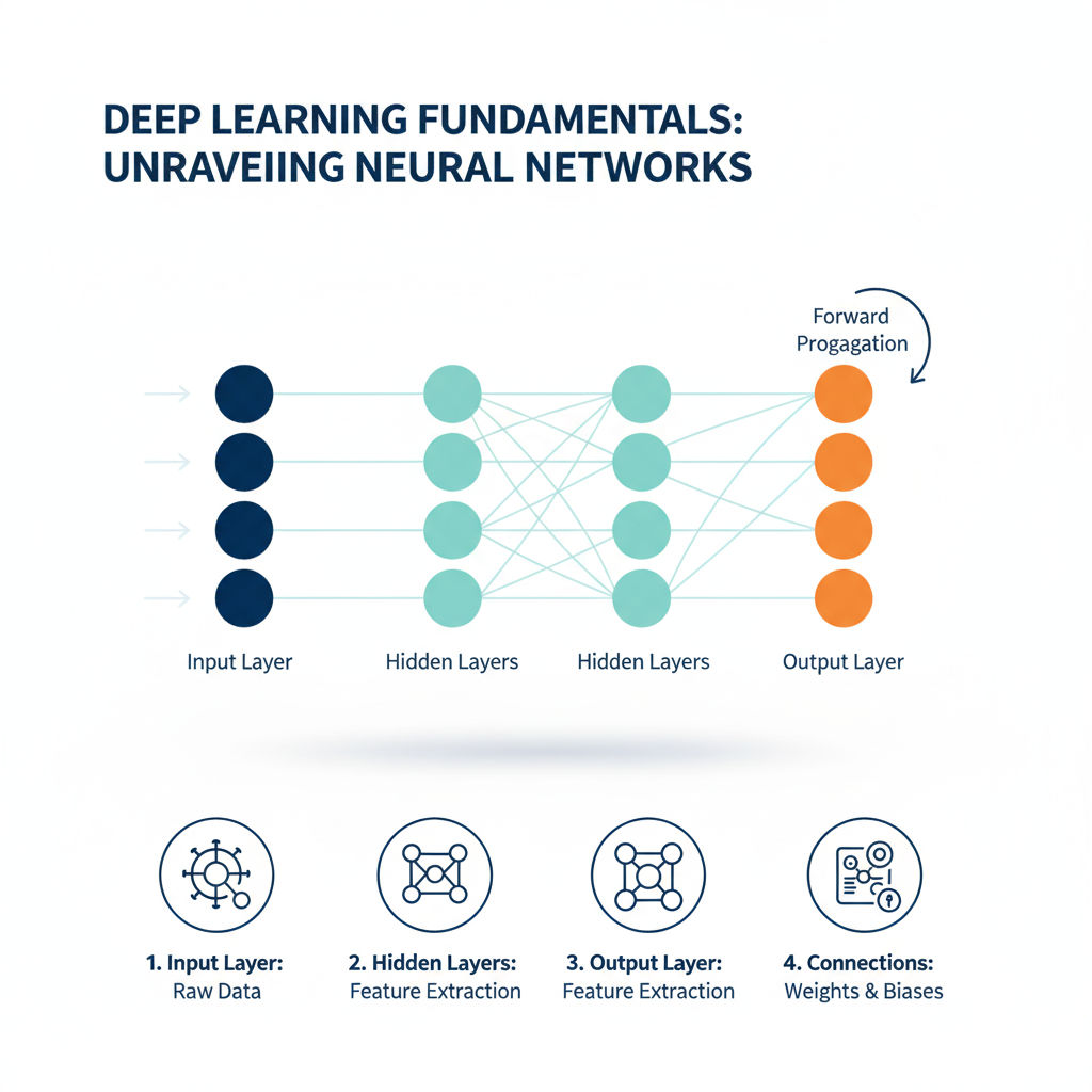
The Multilayer Perceptron (MLP) is the simplest and most fundamental type of Neural Network. It is a class of feedforward neural network composed of at least three layers: an input layer, one or more hidden layers, and an output layer. The “feedforward” designation means that data flows in one direction, from input to output, without any cycles or loops.

The power of the MLP stems from the universal approximation theorem, which states that a feedforward network with a single hidden layer containing a finite number of neurons can approximate any continuous function on compact subsets of Rⁿ, under mild assumptions on the activation function. In essence, given enough Neural Network computational units, an MLP can learn any complex mapping from inputs to outputs.

Architectural Deep Dive:
An MLP’s architecture is defined by its layers and the connections between them.

• Input Layer: This layer represents the features of your dataset. Each node (neuron) corresponds to one feature. For example, in a housing price prediction model, nodes could represent square footage, number of bedrooms, and zip code.
• Hidden Layers: These are the computational engines of the network. Each neuron in a hidden layer receives inputs from all neurons in the previous layer, computes a weighted sum, adds a bias term, and then passes the result through a non-linear activation function. This non-linearity is crucial; without it, the entire network would collapse into a single linear transformation. Common activation functions include ReLU (Rectified Linear Unit), Sigmoid, and Tanh.
• Output Layer: The final layer produces the network’s prediction. Its design is problem-dependent. For binary classification, it often has a single neuron with a sigmoid activation. For multi-class classification, it has multiple neurons (one per class) with a softmax activation. For regression, it typically has a single neuron with a linear or ReLU activation.

The “learning” process, known as backpropagation, involves calculating the error between the prediction and the actual target, then propagating this error backward through the network to adjust the weights and biases using an optimization algorithm like Gradient Descent. This iterative process gradually minimizes the error.

Typical Applications:

• Tabular Data Classification and Regression: Customer churn prediction, credit scoring, real estate price estimation.
• Simple Pattern Recognition: Non-linear trend forecasting in business metrics.
• Foundation for More Complex Systems: Often used as the final classification layer in more complex architectures like Convolutional Neural Networks.

Python Implementation with Keras:

python

import tensorflow as tf
from tensorflow.keras.models import Sequential
from tensorflow.keras.layers import Dense, Dropout
from sklearn.datasets import make_classification
from sklearn.model_selection import train_test_split
from sklearn.preprocessing import StandardScaler
#Neural Network
# Generate a sample dataset
X, y = make_classification(n_samples=1000, n_features=20, n_informative=15, n_redundant=5, n_classes=2, random_state=42)

# Preprocess: Split and Standardize
X_train, X_test, y_train, y_test = train_test_split(X, y, test_size=0.2, random_state=42)
scaler = StandardScaler()
X_train = scaler.fit_transform(X_train)
X_test = scaler.transform(X_test)

# Define the MLP Model Architecture
model = Sequential([
    Dense(64, activation='relu', input_shape=(X_train.shape[1],)), # First hidden layer
    Dropout(0.3), # Regularization to prevent overfitting
    Dense(32, activation='relu'), # Second hidden layer
    Dropout(0.3),
    Dense(1, activation='sigmoid') # Output layer for binary classification
])

# Compile the Model
model.compile(optimizer='adam',
              loss='binary_crossentropy',
              metrics=['accuracy'])

# Train the Model
history = model.fit(X_train, y_train,
                    epochs=100,
                    batch_size=32,
                    validation_split=0.2,
                    verbose=1)

# Evaluate the Model
test_loss, test_accuracy = model.evaluate(X_test, y_test, verbose=0)
print(f"Test Accuracy: {test_accuracy:.4f}")

Part 2: Architectures for Spatial and Visual Intelligence

The real world is rich with spatial and visual data. The following architectures were specifically designed to process this type of information efficiently.

2. Convolutional Neural Network (CNN): The Vision Specialist

Conceptual Foundation:
The Convolutional Neural Network (CNN or ConvNet) is a specialized kind of Neural Network designed for processing data that has a grid-like topology, such as images (a 2D grid of pixels) or time-series data (a 1D grid of time steps). Its revolutionary design was inspired by the organization of the animal visual cortex. The core innovation of CNNs is the use of convolutional layers, which apply a series of filters (also called kernels) to the input data to extract hierarchical features. This allows the network to be spatially invariant, meaning it can recognize an object regardless of its location in the image.

Architectural Deep Dive:
A standard CNN architecture is a sequence of convolutional and pooling layers, followed by fully connected (MLP) layers.

• Convolutional Layer: This is the fundamental building block. It consists of multiple filters that slide (convolve) across the input. Each filter detects a specific feature, such as an edge, a corner, or a texture in a specific orientation. Early layers learn simple features, while deeper layers combine these to learn complex patterns like shapes, objects, and even faces.
• Pooling Layer (Subsampling): Typically inserted between convolutional layers, its purpose is to progressively reduce the spatial size (width and height) of the representation. This reduces the computational load, the number of parameters, and helps to control overfitting. The most common type is Max Pooling, which takes the maximum value from a cluster of neurons.
• Flatten Layer: After the series of convolutional and pooling layers, the high-level reasoning is done via fully connected layers. The Flatten layer converts the 2D feature maps into a 1D vector to feed into the subsequent MLP.
• Fully Connected Layer: These layers, identical to those in an MLP, use the high-level features extracted by the convolutional base to perform the final classification or regression.

This hierarchical feature learning process—from edges to textures to object parts to full objects—is what makes CNNs so powerful for visual tasks.

Typical Applications:

• Image Classification: Identifying the main object in an image (e.g., “cat,” “dog,” “car”).
• Object Detection: Not just classifying, but also locating multiple objects within an image (e.g., YOLO, SSD).
• Semantic Segmentation: Assigning a class label to every single pixel in an image (e.g., for medical imaging or self-driving cars).
• Image Generation: Using variants like Generative Adversarial Networks (GANs) and Variational Autoencoders (VAEs).

Python Implementation with Keras:

python

import tensorflow as tf
from tensorflow.keras import datasets, layers, models
#Neural Network
# Load and preprocess the CIFAR-10 dataset
(train_images, train_labels), (test_images, test_labels) = datasets.cifar10.load_data()
# Normalize pixel values to be between 0 and 1
train_images, test_images = train_images / 255.0, test_images / 255.0

# Define the CNN Model Architecture
model = models.Sequential()
# First Convolutional Block
model.add(layers.Conv2D(32, (3, 3), activation='relu', input_shape=(32, 32, 3)))
model.add(layers.MaxPooling2D((2, 2)))
# Second Convolutional Block
model.add(layers.Conv2D(64, (3, 3), activation='relu'))
model.add(layers.MaxPooling2D((2, 2)))
# Third Convolutional Block
model.add(layers.Conv2D(64, (3, 3), activation='relu'))
# Flatten and use Dense layers for classification
model.add(layers.Flatten())
model.add(layers.Dense(64, activation='relu'))
model.add(layers.Dense(10, activation='softmax')) # 10 classes for CIFAR-10

# Compile the Model
model.compile(optimizer='adam',
              loss='sparse_categorical_crossentropy',
              metrics=['accuracy'])

# Train the Model
history = model.fit(train_images, train_labels,
                    epochs=10,
                    validation_data=(test_images, test_labels))

# Evaluate the Model
test_loss, test_accuracy = model.evaluate(test_images, test_labels, verbose=2)
print(f"Test Accuracy: {test_accuracy:.4f}")

3. Autoencoder (AE): The Data Compression and Denoising Engine

Conceptual Foundation:
An Autoencoder is a type of Neural Network used for unsupervised learning. Its primary goal is to learn an efficient, compressed representation (encoding) of the input data. The network is trained to reconstruct its own input, which may seem trivial, but the “bottleneck” in the middle forces it to learn the most important aspects of the data. Think of it as a powerful, non-linear form of dimensionality reduction, like PCA on steroids.

Architectural Deep Dive:
An autoencoder consists of two main parts:

• Encoder: This part of the network compresses the input into a latent-space representation. It typically consists of a series of layers that progressively reduce the dimensionality (e.g., Dense layers with fewer units or Convolutional layers with pooling).
• Bottleneck (Latent Space): This is the layer that contains the compressed knowledge of the input data. It is the most crucial part of the network. Its low dimensionality creates an “information bottleneck,” forcing the encoder to learn a smart, compressed representation.
• Decoder: This part of the network aims to reconstruct the input data from the latent space representation. It mirrors the encoder’s architecture, progressively upsampling the data back to its original dimensions.

The network is trained by minimizing a reconstruction loss, such as Mean Squared Error (MSE) or Binary Cross-Entropy, which measures the difference between the original input and the reconstructed output.

Typical Applications:

• Dimensionality Reduction: A non-linear alternative to PCA.
• Image Denoising: Train the autoencoder on clean images, but feed it noisy images during training. It learns to output clean versions.
• Anomaly Detection: After training on “normal” data, the autoencoder will be poor at reconstructing anomalous data. A high reconstruction error indicates an anomaly.
• Feature Learning: The encoder can be used as a pre-processing step to learn features for a subsequent supervised task.

Python Implementation with Keras:

python

import tensorflow as tf
from tensorflow.keras import layers, Model
import numpy as np
import matplotlib.pyplot as plt
#Neural Network
# Use MNIST for a simple demonstration
(x_train, _), (x_test, _) = tf.keras.datasets.mnist.load_data() # We don't need the labels
x_train = x_train.astype('float32') / 255.
x_test = x_test.astype('float32') / 255.
x_train = x_train.reshape((len(x_train), 28, 28, 1))
x_test = x_test.reshape((len(x_test), 28, 28, 1))

# Add noise to the images for a denoising example
noise_factor = 0.5
x_train_noisy = x_train + noise_factor * np.random.normal(loc=0.0, scale=1.0, size=x_train.shape)
x_test_noisy = x_test + noise_factor * np.random.normal(loc=0.0, scale=1.0, size=x_test.shape)
x_train_noisy = np.clip(x_train_noisy, 0., 1.)
x_test_noisy = np.clip(x_test_noisy, 0., 1.)

# Define the Encoder
input_img = layers.Input(shape=(28, 28, 1))
x = layers.Conv2D(32, (3, 3), activation='relu', padding='same')(input_img)
x = layers.MaxPooling2D((2, 2), padding='same')(x)
x = layers.Conv2D(32, (3, 3), activation='relu', padding='same')(x)
encoded = layers.MaxPooling2D((2, 2), padding='same')(x) # Bottleneck: 7x7x32

# Define the Decoder
x = layers.Conv2D(32, (3, 3), activation='relu', padding='same')(encoded)
x = layers.UpSampling2D((2, 2))(x)
x = layers.Conv2D(32, (3, 3), activation='relu', padding='same')(x)
x = layers.UpSampling2D((2, 2))(x)
decoded = layers.Conv2D(1, (3, 3), activation='sigmoid', padding='same')(x)

# Create the Autoencoder model
autoencoder = Model(input_img, decoded)
autoencoder.compile(optimizer='adam', loss='binary_crossentropy')

# Train the model to reconstruct the clean images from the noisy ones
autoencoder.fit(x_train_noisy, x_train, # Input: noisy, Target: clean
                epochs=10,
                batch_size=128,
                shuffle=True,
                validation_data=(x_test_noisy, x_test))
#Neural Network
# Visualize the denoising results
decoded_imgs = autoencoder.predict(x_test_noisy)
n = 5
plt.figure(figsize=(10, 4))
for i in range(n):
    # Display noisy input
    ax = plt.subplot(2, n, i + 1)
    plt.imshow(x_test_noisy[i].reshape(28, 28), cmap='gray')
    # Display reconstruction
    ax = plt.subplot(2, n, i + 1 + n)
    plt.imshow(decoded_imgs[i].reshape(28, 28), cmap='gray')
plt.show()

Part 3: Architectures for Sequential and Temporal Data

Data that exists in a sequence, where the order matters, requires a different architectural approach. These networks have a “memory” of previous inputs.

4. Recurrent Neural Network (RNN): The Sequential Data Pioneer

Conceptual Foundation:
Recurrent Neural Networks (RNNs) are a class of Neural Networks designed specifically for sequential data. Unlike feedforward networks, RNNs have connections that form directed cycles, allowing them to maintain a “hidden state” that acts as a memory of previous inputs in the sequence. This makes them theoretically well-suited for tasks where context from earlier in the sequence is crucial for understanding the current element, such as in time series forecasting or natural language processing.

Architectural Deep Dive:
The key feature of an RNN is its recurrent cell, which is applied to each element in the sequence.

• The Recurrent Cell: At each time step t, the cell receives two inputs: the current data point x_t and its own hidden state from the previous time step h_{t-1}. It then computes a new hidden state h_t and an output y_t.
• Parameter Sharing: The same set of weights and biases (the RNN cell’s parameters) are used at every time step. This makes the model efficient and allows it to be applied to sequences of different lengths.
• Unfolding the RNN: To visualize and understand the flow of information, an RNN can be “unfolded” in time, creating a deep feedforward network where each layer corresponds to a time step. This unfolding also reveals the central challenge of training RNNs: the vanishing/exploding gradient problem. During backpropagation through time (BPTT), gradients are multiplied repeatedly by the same weight matrix. If these weights are small, the gradient can vanish, preventing learning of long-range dependencies. If they are large, the gradient can explode.

Typical Applications:

• Time Series Forecasting: Predicting stock prices, weather, or energy demand.
• Language Modeling: Predicting the next word in a sentence.
• Basic Text Classification: Sentiment analysis at the document level.

Python Implementation with Keras:

python

import tensorflow as tf
from tensorflow.keras.models import Sequential
from tensorflow.keras.layers import SimpleRNN, Dense
import numpy as np
#Neural Network
# Generate a simple synthetic sequential dataset
def generate_sequence_data(n_samples, sequence_length, n_features):
    X = np.random.randn(n_samples, sequence_length, n_features)
    # Simple target: 1 if the sum of the first feature in the sequence is positive, else 0
    y = (np.sum(X[:, :, 0], axis=1) > 0).astype(int)
    return X, y
#Neural Network
X, y = generate_sequence_data(1000, 10, 5) # 1000 samples, 10 time steps, 5 features per step

# Define a Simple RNN Model
model = Sequential([
    # SimpleRNN layer with 50 units. `return_sequences=False` means it only returns the last output.
    SimpleRNN(50, activation='relu', input_shape=(X.shape[1], X.shape[2])),
    Dense(1, activation='sigmoid') # Output layer for binary classification
])
#Neural Network
model.compile(optimizer='adam', loss='binary_crossentropy', metrics=['accuracy'])
#Neural Network
# Train the model
history = model.fit(X, y, epochs=20, batch_size=32, validation_split=0.2, verbose=1)

# Evaluate
test_loss, test_accuracy = model.evaluate(X, y, verbose=0)
print(f"Test Accuracy: {test_accuracy:.4f}")

5. Long Short-Term Memory (LSTM): Mastering Long-Range Dependencies

Conceptual Foundation:
The Long Short-Term Memory (LSTM) network is a special kind of RNN, specifically engineered to address the vanishing gradient problem and to learn long-range dependencies. Introduced by Sepp Hochreiter and Jürgen Schmidhuber in 1997, LSTMs have become one of the most widely used and successful architectures for sequence modeling. They are capable of remembering information for long periods of time, which is often critical for understanding context in language or patterns in long time series.

Architectural Deep Dive:
The LSTM’s secret sauce is its sophisticated cell structure, which includes a “cell state” that runs through the entire sequence chain, like a conveyor belt. Information can be added or removed from this cell state via three regulatory mechanisms called “gates.”

• Cell State (C_t): The horizontal line that runs through the top of the cell. It carries information along the entire sequence, with minor linear interactions. It is the long-term memory.
• Forget Gate (f_t): A sigmoid layer that looks at the previous hidden state h_{t-1} and the current input x_t, and outputs a number between 0 and 1 for each number in the cell state C_{t-1}. A 1 means “completely keep this,” while a 0 means “completely forget this.”
• Input Gate (i_t) and Candidate Cell State (~C_t): The input gate decides which values of the candidate cell state we’ll update. The candidate cell state ~C_t is a new vector created from the current input and previous hidden state via a tanh layer, containing potential new information.
• Output Gate (o_t): This gate decides what the next hidden state h_t should be. The hidden state is a filtered version of the cell state and is used for predictions.

This gated architecture allows the LSTM to selectively remember or forget information, making it remarkably effective for tasks requiring long-term context.

Typical Applications:

• Machine Translation: Powering models like Google Translate.
• Speech Recognition: Transcribing audio to text.
• Text Generation: Writing articles, code, or poetry.
• Video Analysis: Understanding actions across multiple frames.

Python Implementation with Keras:

python

import tensorflow as tf
from tensorflow.keras.datasets import imdb
from tensorflow.keras.preprocessing import sequence
from tensorflow.keras.models import Sequential
from tensorflow.keras.layers import Embedding, LSTM, Dense

# Load the IMDB movie review sentiment dataset
max_features = 10000  # Only consider the top 10,000 words
maxlen = 500  # Only consider the first 500 words of each review
#Neural Network
(x_train, y_train), (x_test, y_test) = imdb.load_data(num_words=max_features)
print(f"Training sequence: {len(x_train)}, Test sequences: {len(x_test)}")

# Pad sequences to ensure uniform length
x_train = sequence.pad_sequences(x_train, maxlen=maxlen)
x_test = sequence.pad_sequences(x_test, maxlen=maxlen)
#Neural Network
# Define the LSTM Model for Sentiment Analysis
model = Sequential([
    # Embedding layer turns word indices into dense vectors of fixed size
    Embedding(max_features, 128),
    # LSTM layer with 64 units. We can use `return_sequences=True` to stack LSTMs.
    LSTM(64, dropout=0.2, recurrent_dropout=0.2),
    # Output layer for binary classification (positive/negative sentiment)
    Dense(1, activation='sigmoid')
])
#Neural Network
model.compile(optimizer='adam',
              loss='binary_crossentropy',
              metrics=['accuracy'])

# Train the model
history = model.fit(x_train, y_train,
                    batch_size=32,
                    epochs=5,
                    validation_data=(x_test, y_test))
#Neural Network
# Evaluate
test_loss, test_accuracy = model.evaluate(x_test, y_test, verbose=0)
print(f"Test Accuracy: {test_accuracy:.4f}")

6. Gated Recurrent Unit (GRU): The LSTM’s Efficient Sibling

Conceptual Foundation:
The Gated Recurrent Unit (GRU) is a more recent evolution of the RNN, introduced in 2014 as a simplification of the LSTM. It combines the forget and input gates into a single “update gate.” It also merges the cell state and hidden state. The result is a model that is often just as effective as an LSTM but is computationally cheaper and faster to train, as it has fewer parameters.

Architectural Deep Dive:
The GRU cell contains two gates:

• Update Gate (z_t): This gate decides how much of the past information (from previous hidden states) needs to be passed along to the future. It replaces the LSTM’s forget and input gates. It acts as a blend, deciding what to forget and what new information to add.
• Reset Gate (r_t): This gate determines how much of the past information to forget. It allows the model to drop information that is irrelevant in the future, helping it to capture short-term dependencies.

The simplified architecture makes GRUs a popular choice when computational efficiency is important and when the sequence lengths are not extremely long.

Typical Applications:

• Same as LSTM, but preferred when: Training speed and resource efficiency are critical.
• Language Modeling: Next-character or next-word prediction.
• Polyphonic Music Modeling: Predicting multiple notes in a musical score.

Python Implementation with Keras:

python

import tensorflow as tf
from tensorflow.keras.models import Sequential
from tensorflow.keras.layers import GRU, Dense, Embedding
from tensorflow.keras.datasets import imdb
from tensorflow.keras.preprocessing import sequence
#Neural Network
# Using the same IMDB dataset as before
max_features = 10000
maxlen = 500
#Neural Network
(x_train, y_train), (x_test, y_test) = imdb.load_data(num_words=max_features)
x_train = sequence.pad_sequences(x_train, maxlen=maxlen)
x_test = sequence.pad_sequences(x_test, maxlen=maxlen)

# Define the GRU Model
model = Sequential([
    Embedding(max_features, 128),
    GRU(64, dropout=0.2, recurrent_dropout=0.2), # Using GRU instead of LSTM
    Dense(1, activation='sigmoid')
])

model.compile(optimizer='adam',
              loss='binary_crossentropy',
              metrics=['accuracy'])
#Neural Network
# Train the model
history = model.fit(x_train, y_train,
                    batch_size=32,
                    epochs=5,
                    validation_data=(x_test, y_test))
#Neural Network
# Evaluate
test_loss, test_accuracy = model.evaluate(x_test, y_test, verbose=0)
print(f"GRU Test Accuracy: {test_accuracy:.4f}")

Part 4: The Modern Transformer Revolution

The Transformer architecture, introduced in 2017, has fundamentally reshaped the field of NLP and beyond, moving away from recurrence and towards a mechanism of pure attention.

7. Transformer: The Architecture That Changed Everything

Conceptual Foundation:
The Transformer, introduced in the seminal paper “Attention Is All You Need,” completely abandoned the recurrent structure of LSTMs and GRUs. Its core innovation is the self-attention mechanism, which allows the model to weigh the importance of different words in a sequence when encoding a particular word, regardless of their positional distance. This enables direct, parallelized connections across the entire sequence, overcoming the sequential processing bottleneck of RNNs and allowing for massive scaling on modern hardware like GPUs and TPUs.

Architectural Deep Dive:
The Transformer uses an encoder-decoder structure, but its key components are:

• Self-Attention Mechanism: For each word, self-attention produces a representation by taking a weighted sum of the representations of all other words in the sequence. The weights (attention scores) are calculated based on the compatibility between the current word and every other word. This allows the model to focus on relevant context.
• Multi-Head Attention: Instead of performing a single attention function, the Transformer linearly projects the input into multiple different representation subspaces and performs attention in parallel. This allows the model to jointly attend to information from different perspectives (e.g., syntactic and semantic relationships).
• Positional Encoding: Since the Transformer contains no recurrence or convolution, it has no inherent notion of word order. Positional encodings are added to the input embeddings to inject information about the relative or absolute position of the tokens in the sequence.
• Feed-Forward Networks: After attention, each position is processed independently by the same feed-forward network.
• Residual Connections and Layer Normalization: These are used around each sub-layer to stabilize and accelerate training.

Typical Applications:

• Machine Translation: The original application.
• Text Summarization: Creating concise summaries of long documents.
• BERT and GPT Models: The foundational architecture for all modern large language models.

Python Implementation (Conceptual with TensorFlow):
Note: A full Transformer implementation is complex. Here is a simplified snippet for the Multi-Head Attention mechanism, its core component.

python

import tensorflow as tf
#Neural Network
def scaled_dot_product_attention(query, key, value, mask=None):
    """Calculate the attention weights."""
    matmul_qk = tf.matmul(query, key, transpose_b=True)
    # scale matmul_qk
    depth = tf.cast(tf.shape(key)[-1], tf.float32)
    logits = matmul_qk / tf.math.sqrt(depth)
    # add the mask to zero out padding tokens (if provided)
    if mask is not None:
        logits += (mask * -1e9)
    # softmax is normalized on the last axis (seq_len_k)
    attention_weights = tf.nn.softmax(logits, axis=-1)
    output = tf.matmul(attention_weights, value)
    return output, attention_weights
#Neural Network
# Example of using the function (conceptual)
# Let's assume we have embeddings for a sequence of 4 words, each of dimension 64.
batch_size = 1
seq_len = 4
d_model = 64
query = tf.random.normal((batch_size, seq_len, d_model))
key = tf.random.normal((batch_size, seq_len, d_model))
value = tf.random.normal((batch_size, seq_len, d_model))
#Neural Network
output, attention_weights = scaled_dot_product_attention(query, key, value)
print(f"Output shape: {output.shape}")  # (1, 4, 64)
print(f"Attention weights shape: {attention_weights.shape}")  # (1, 4, 4)
# The attention weights show how much each word (4) attends to every other word (4).

8. Generative Adversarial Network (GAN): The Creative Artist

Conceptual Foundation:
Generative Adversarial Networks (GANs), introduced by Ian Goodfellow in 2014, represent a breakthrough in generative modeling. Instead of having a single network that learns to generate data, a GAN pits two Neural Networks against each other in a game-theoretic framework:

• The Generator: Takes random noise as input and tries to generate fake data (e.g., an image) that is indistinguishable from real data.
• The Discriminator: Takes both real data and the fake data from the generator and tries to correctly classify them as “real” or “fake.”

The two networks are trained simultaneously in an adversarial process: the generator is learning to produce more convincing fakes, while the discriminator is learning to become a better detective. This competition drives both networks to improve until the generator produces highly realistic data.

Architectural Deep Dive:
The training process is a minimax game. The generator aims to minimize the discriminator’s ability to detect fakes, while the discriminator aims to maximize it.

1. Phase 1 – Train Discriminator: A batch of real images is sampled from the dataset and labeled “real.” A batch of fake images is generated from random noise and labeled “fake.” The discriminator is trained on this combined batch to improve its classification accuracy.
2. Phase 2 – Train Generator: New random noise is generated and passed through the generator to create fake images. This time, the discriminator is frozen, and the entire composite model (generator -> discriminator) is trained. The generator’s weights are updated to fool the discriminator, i.e., to make it output “real” for the fake images.

This process is repeated iteratively. Finding the right balance (Nash equilibrium) is challenging, and GAN training is famously unstable.

Typical Applications:

• Image Generation: Creating photorealistic images of human faces, animals, and scenes (e.g., StyleGAN).
• Image-to-Image Translation: Converting satellite photos to maps, day photos to night, sketches to photos (e.g., Pix2Pix, CycleGAN).
• Data Augmentation: Generating synthetic training data for other models.
• Super-Resolution: Increasing the resolution of low-quality images.

Python Implementation with Keras (DCGAN for MNIST):

python

import tensorflow as tf
from tensorflow.keras import layers, Model
import numpy as np
import matplotlib.pyplot as plt
#Neural Network
# Define the Generator
def make_generator_model():
    model = tf.keras.Sequential()
    model.add(layers.Dense(7*7*256, use_bias=False, input_shape=(100,)))
    model.add(layers.BatchNormalization())
    model.add(layers.LeakyReLU())
    model.add(layers.Reshape((7, 7, 256)))
    # Upsample to 14x14
    model.add(layers.Conv2DTranspose(128, (5, 5), strides=(1, 1), padding='same', use_bias=False))
    model.add(layers.BatchNormalization())
    model.add(layers.LeakyReLU())
    # Upsample to 28x28
    model.add(layers.Conv2DTranspose(64, (5, 5), strides=(2, 2), padding='same', use_bias=False))
    model.add(layers.BatchNormalization())
    model.add(layers.LeakyReLU())
    # Output layer
    model.add(layers.Conv2DTranspose(1, (5, 5), strides=(2, 2), padding='same', use_bias=False, activation='tanh'))
    return model

# Define the Discriminator
def make_discriminator_model():
    model = tf.keras.Sequential()
    model.add(layers.Conv2D(64, (5, 5), strides=(2, 2), padding='same', input_shape=[28, 28, 1]))
    model.add(layers.LeakyReLU())
    model.add(layers.Dropout(0.3))
    model.add(layers.Conv2D(128, (5, 5), strides=(2, 2), padding='same'))
    model.add(layers.LeakyReLU())
    model.add(layers.Dropout(0.3))
    model.add(layers.Flatten())
    model.add(layers.Dense(1, activation='sigmoid')) # Outputs a probability (real/fake)
    return model
#Neural Network
# Instantiate models
generator = make_generator_model()
discriminator = make_discriminator_model()
#Neural Network
# Define loss and optimizers
cross_entropy = tf.keras.losses.BinaryCrossentropy()
generator_optimizer = tf.keras.optimizers.Adam(1e-4)
discriminator_optimizer = tf.keras.optimizers.Adam(1e-4)
#Neural Network
# Training step (simplified outline)
@tf.function
def train_step(images):
    noise = tf.random.normal([BATCH_SIZE, 100])
    with tf.GradientTape() as gen_tape, tf.GradientTape() as disc_tape:
        generated_images = generator(noise, training=True)
        real_output = discriminator(images, training=True)
        fake_output = discriminator(generated_images, training=True)
        gen_loss = generator_loss(fake_output)
        disc_loss = discriminator_loss(real_output, fake_output)
    gradients_of_generator = gen_tape.gradient(gen_loss, generator.trainable_variables)
    gradients_of_discriminator = disc_tape.gradient(disc_loss, discriminator.trainable_variables)
    generator_optimizer.apply_gradients(zip(gradients_of_generator, generator.trainable_variables))
    discriminator_optimizer.apply_gradients(zip(gradients_of_discriminator, discriminator.trainable_variables))
#Neural Network
# Note: The full training loop, loss functions, and visualization code are more extensive.
# This snippet provides the core architectural definition.

Part 5: Advanced and Hybrid Architectures

The most powerful modern systems often combine ideas from multiple architectures or are designed for specific, complex tasks.

9. Graph Neural Network (GNN): Reasoning About Relationships

Conceptual Foundation:
Graph Neural Networks (GNNs) are a class of Neural Networks designed to perform inference on data described by graphs. A graph is a structure consisting of nodes (vertices) and edges (connections). This is a highly general and powerful representation; molecules are graphs (atoms and bonds), social networks are graphs (users and friendships), and knowledge