Mastering Bayes Theorem: Conditional Probability Made Easy

Master Bayes Theorem: Learn how to update beliefs with evidence. Essential for AI, data science, and rational thinking. Your guide to conditional probability

Introduction: The Theorem That Changed the World

Imagine a tool so powerful that it forms the bedrock of modern artificial intelligence, a principle so elegant that it deciphers the mysteries of human cognition, and a formula so practical that it helps doctors diagnose diseases and engineers build spam filters. This is not a futuristic fantasy; it is the reality of Bayes theorem.

At its heart, Bayes theorem is a formal, mathematical way to update our beliefs in the face of new evidence. It is a framework for navigating a world of uncertainty, allowing us to move from initial assumptions to more informed conclusions. For centuries, this theorem, formulated by the Reverend Thomas Bayes in the 18th century, was a curious niche in probability theory. Today, it is nothing short of a revolutionary force.

Yet, for many, the very mention of Bayes theorem conjures images of impenetrable equations and abstract statistical concepts. This article aims to dismantle that perception. We will embark on a journey to not just understand but to truly master Bayes theorem. We will strip it down to its intuitive core, explore its myriad applications with concrete examples, and demonstrate why it is arguably the most important statistical concept for the 21st century. By the end of this guide, conditional probability will not just be easy—it will be a fundamental part of your analytical toolkit.

Part 1: Laying the Foundation – Probability, Conditionality, and the Inverse

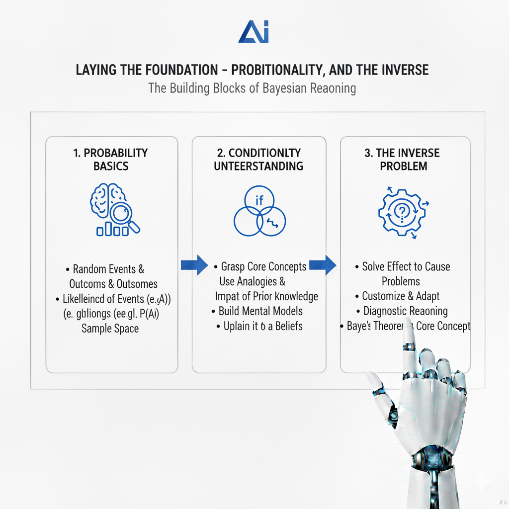
To build a skyscraper, you need a solid foundation. To master Bayes theorem, you must first be comfortable with the concepts of probability, conditional probability, and the critical difference between two often-confused directions of reasoning.

1.1 A Quick Refresher: What is Probability?

Probability is the language of uncertainty. It quantifies how likely an event is to occur, represented as a number between 0 and 1 (or 0% and 100%).

• P(A) = 0: The event A is impossible.
• P(A) = 1: The event A is certain.
• P(A) = 0.3: The event A has a 30% chance of happening.

The sum of the probabilities of all possible Bayes theorem mutually exclusive outcomes for a given scenario is always 1.

1.2 The Game-Changer: Conditional Probability

Conditional probability is the probability of an event given that another event has already occurred. This is the “if-then” of probability and the cornerstone of Bayes theorem.

The notation is P(A|B), read as “the probability of A given B.” It asks: “Now that we know B has happened, how does that change the probability of A happening?”

Example: The Rain and Cloud Scenario

• Let A be the event “it rains.”
• Let B be the event “there are clouds in the sky.”
• P(A), the probability of rain on any given day, might be 0.2 (20%).
• P(A|B), the probability of rain given that there are clouds, is much higher, say 0.8 (80%).

The condition “given clouds” dramatically Bayes theorem updates our belief about the likelihood of rain. This updating is the essence of learning from evidence.

The formula for conditional probability is:

P(A|B) = P(A and B) / P(B)

This makes intuitive sense. To find the probability of A given B, we look at the probability that both A and B happen (the joint probability) and then restrict it to the world where B is already true (divided by P(B)).

1.3 The Critical Confusion: P(A|B) vs. P(B|A)

This is the single most important hurdle to clear. P(A|B) and P(B|A) are not the same thing! Confusing them is a logical error known as the “inverse fallacy” or “prosecutor’s fallacy,” and it has led to grave miscarriages of justice.

Let’s illustrate with a classic medical example.

• A: The patient has a specific disease.
• B: The patient tests positive for the disease.
• P(B|A): The probability of testing positive given that you have the disease. This is the sensitivity of the test. A good test Bayes theorem has a high sensitivity, say 0.99 (99%).
• P(A|B): The probability of having the disease given that you tested positive. This is what a patient who just got a positive result desperately wants to know.

These are fundamentally different questions. P(B|A) is a property of the test. P(A|B) depends not only on the test’s accuracy but also on how common the disease, P(A), is in the population. If the disease is very rare, even a positive result from a great test might not mean you’re likely to have it. We will solve this exact problem with Bayes theorem shortly.

Part 2: Unveiling the Magic – Deriving and Understanding Bayes Theorem

Now that we have a deep understanding of conditional probability and the perils of confusing the inverse, we are ready to meet the theorem that elegantly connects them.

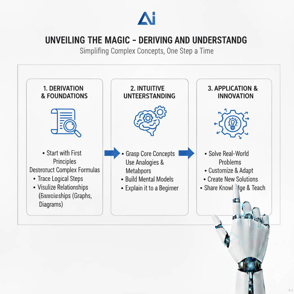
2.1 The Formal Derivation from First Principles

We start with the definition of conditional probability, written in two symmetrical ways:

1. P(A|B) = P(A and B) / P(B)
2. P(B|A) = P(A and B) / P(A)

Notice that both equations share the term P(A and B), the joint probability of both events occurring. Let’s solve for this joint probability from each equation:

From (1): P(A and B) = P(A|B) * P(B)
From (2): P(A and B) = P(B|A) * P(A)

Since both expressions on the right are equal to P(A and B), we can set them equal to each other:

P(B|A) * P(A) = P(A|B) * P(B)

This is a powerful statement: it shows the relationship between the two conditional probabilities. Finally, to solve for the quantity we often want, P(A|B), we can divide both sides by P(B):

P(A|B) = [P(B|A) * P(A)] / P(B)

And there it is. Bayes Theorem in its simplest form.

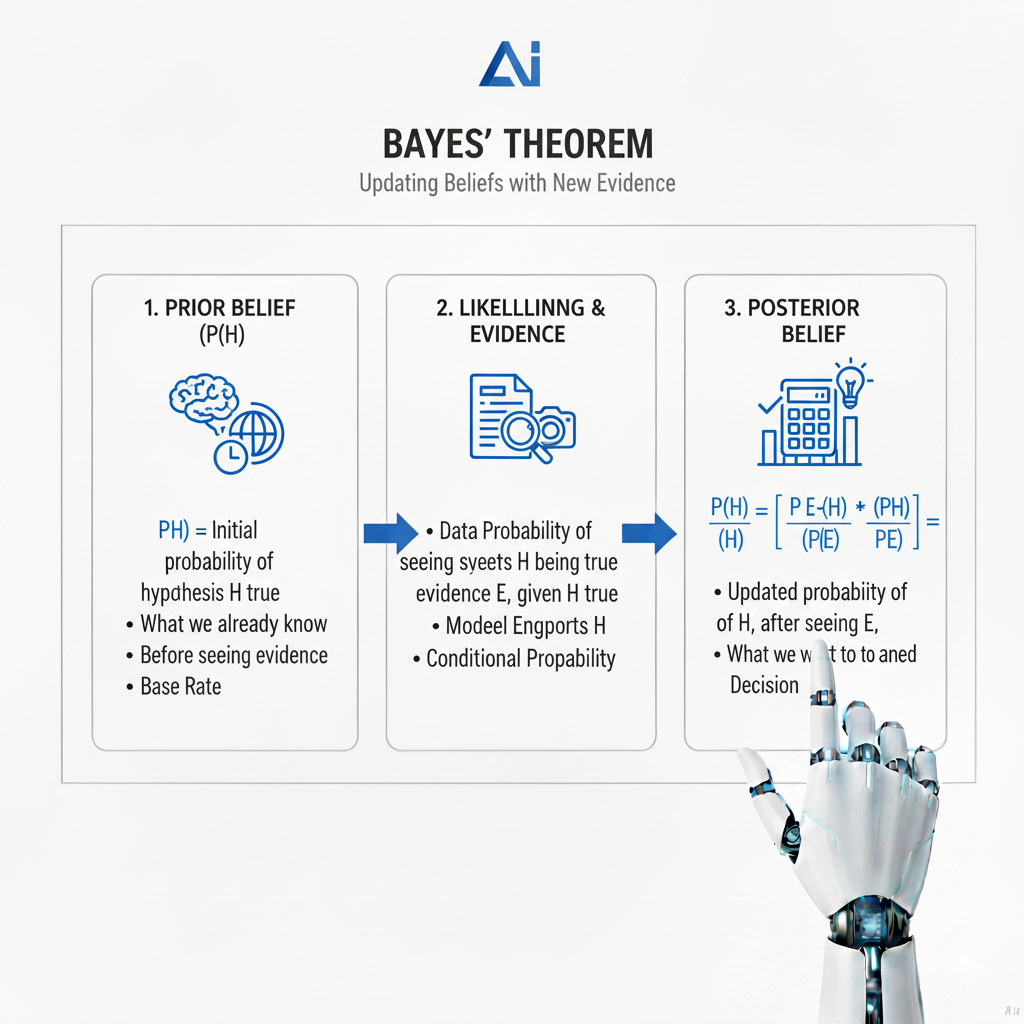
2.2 The Core Components and Their Philosophical Meaning

Bayes theorem is more than a formula; it’s a recipe for rational thinking. Each component has a specific name and a profound philosophical meaning, Bayes theorem transforming it from an equation into a model for learning.

• P(A) – The Prior Probability (The Initial Belief)
  This is our initial degree of belief in hypothesis A before seeing the new evidence B. It can be based on historical data, expert opinion, a logical assumption, or even a subjective guess. The prior is often the most controversial but also the most powerful part of Bayesian analysis, as it formally incorporates existing knowledge. In the medical example, it’s the base rate of the disease. In the legal example, it’s the prior assumption of innocence. Ignoring the prior is the root of the base rate fallacy.
• P(B|A) – The Likelihood (The Evidence’s Strength)
  This is the probability of observing evidence B given that our hypothesis A is true. It is not a probability distribution over A, but a function of B. It tells us how “compatible” or “likely” the observed evidence is under our hypothesis. A high likelihood means the evidence is very plausible if our hypothesis is correct. In the medical test, this is the sensitivity. In the DNA example, this is the 1 in 1,000,000 probability of a match given innocence.
• P(B) – The Marginal Likelihood or Evidence (The Total Probability of the Evidence)
  This is the total probability of observing evidence B under all possible hypotheses. It acts as a normalizing constant, ensuring the posterior probability is a valid value between 0 and 1. It can be calculated using the law of total probability, which we saw earlier: P(B) = P(B|A) * P(A) + P(B|not A) * P(not A). This accounts for all ways the evidence could occur, both if A is true and if A is false. It’s the denominator that ensures our updated belief is properly calibrated against the entirety of the available information.
• P(A|B) – The Posterior Probability (The Updated Belief)
  This is the output of the theorem and the ultimate goal. It represents our revised belief about hypothesis A after taking into account the new evidence B. The process is cyclical: today’s posterior becomes tomorrow’s prior. This sequential updating is what allows for continuous learning and refinement of beliefs as new data streams in.

The Bayesian Philosophy of Learning: The theorem provides a mathematical model for scientific reasoning and human learning. We start with a Prior belief, however vague. We then collect new Evidence. We evaluate the strength of this evidence via the Likelihood. We then combine these, normalizing by the total probability Bayes theorem of the evidence, to arrive at a new, updated Posterior belief. This process is iterative. With enough evidence, even wildly different priors held by different people will often converge to the same robust posterior, modeling how scientific consensus is built.

Part 3: Bayes Theorem in Action: From Medical Tests to Machine Intelligence

Theory is essential, but the true power of Bayes theorem is revealed through detailed application. Let’s solve classic and modern problems with step-by-step calculations.

3.1 The Medical Testing Problem – A Comprehensive Solution

Let’s return to and expand upon the medical testing scenario, making it more realistic.

Scenario: A new, highly contagious virus is spreading. You decide to get tested.

• A: You have the virus. (Our hypothesis)
• B: You test positive for the virus. (Our evidence)

Known Information from public health data and test manufacturer:

• The prevalence of the virus in your city, based on widespread testing, is 2%. So, the Prior, P(A) = 0.02. Therefore, P(not A) = 0.98.
• The test has a Sensitivity of 95%. This means if you have the virus, the test will be positive 95% of the time. So, the Likelihood, P(B|A) = 0.95.
• The test has a Specificity of 99%. This means if you do not have the virus, the test will be negative 99% of the time. Therefore, the False Positive Rate, P(B|not A) = 1 – 0.99 = 0.01.

You take the test, and the result comes back POSITIVE. What is the probability you actually have the virus? That is, what is P(A|B)?

Applying Bayes Theorem:

Step 1: Write down the formula.
P(A|B) = [P(B|A) * P(A)] / P(B)

Step 2: Calculate the Numerator.
P(B|A) * P(A) = 0.95 * 0.02 = 0.019

Step 3: Calculate the Denominator, P(B), using the Law of Total Probability.
P(B) = P(B|A) * P(A) + P(B|not A) * P(not A)
P(B) = (0.95 * 0.02) + (0.01 * 0.98)
P(B) = (0.019) + (0.0098) = 0.0288

Step 4: Complete the Calculation.
P(A|B) = 0.019 / 0.0288 ≈ 0.6597

Result: The probability you have the virus, given a positive test, is only about 66%.

This is often a shocking result. Despite the test’s 95% sensitivity and 99% specificity, there is still a 34% chance you are not infected after Bayes theorem a positive result. Why? Because the virus is relatively rare (2% prevalence). The number of false positives (1% of the 98% healthy people) is large enough to contaminate the pool of positive results. This brilliantly demonstrates why understanding Bayes theorem is crucial for interpreting any diagnostic test, especially for rare conditions. It shows that a test’s stated accuracy can be dangerously misleading if not interpreted in context.

3.2 The Intuitive Explanation: Thinking in Populations and Natural Frequencies

Sometimes, abandoning the formula and thinking in whole numbers (natural frequencies) makes Bayes theorem even more transparent and avoids common cognitive errors. Let’s use the same medical example with a hypothetical population.

Let’s assume a city has 1,000,000 people.

• Step 1: Apply the Prior (Prevalence).
  • People with the virus (2%): 0.02 * 1,000,000 = 20,000 people.
  • People without the virus: 980,000 people.
• Step 2: Apply the Likelihood (Test Sensitivity) to the sick group.
  • Of the 20,000 sick people, 95% test positive: 0.95 * 20,000 = 19,000 people. (True Positives)
  • The remaining 1,000 sick people test negative. (False Negatives)
• Step 3: Apply the False Positive Rate to the healthy group.
  • Of the 980,000 healthy people, 1% test positive: 0.01 * 980,000 = 9,800 people. (False Positives)
  • The remaining 970,200 healthy people test negative. (True Negatives)
• Step 4: Find the total number of positive tests.
  • Total Positive Tests = True Positives + False Positives = 19,000 + 9,800 = 28,800 people.
• Step 5: Find the proportion of positive tests that are true positives.
  • This is our desired posterior probability: P(Has Virus | Positive Test) = True Positives / All Positives = 19,000 / 28,800 ≈ 0.6597 or 65.97%.

This population-level grid, often called a contingency table or a Bayesian bucket diagram, perfectly mirrors the calculation from Bayes theorem. It visualizes why the posterior probability is what it is: the “True Positives” bucket is much smaller than the “False Positives” bucket when the disease is rare, even with a good test. This method is highly recommended for building an unshakable intuition.

Part 4: Advanced Applications – How Bayes Theorem Powers the Modern World

The utility of Bayes theorem extends far beyond textbook medical examples. It is the engine behind many of the technologies and methodologies that define our age.

4.1 Spam Filtering: The Classic Example of Naive Bayes

Your email provider uses Bayes theorem thousands of times per second to classify incoming messages. This is typically implemented using a “Naive Bayes” classifier, a powerful and computationally efficient application.

• The Hypothesis (A): “This email is spam.”
• The Evidence (B): The email contains a specific set of words and features (e.g., “free,” “offer,” “viagra,” sender’s address, HTML formatting).

The filter doesn’t just guess; it calculates a probability.

• The Prior, P(Spam): This is the overall proportion of emails that are spam in your inbox (e.g., 30%). The filter learns this from your behavior (marking as spam/not spam).
• The Likelihood, P(Words|Spam): This is the probability that these specific words appear in a known spam email. For example, the word “viagra” might appear in 15% of all spam emails but only 0.001% of non-spam (ham) emails. Bayes theorem The filter learns these likelihoods from a massive training dataset of pre-labeled spam and ham emails. The “Naive” assumption is that the words are independent of each other, which, while not strictly true, simplifies the math and works remarkably well in practice.
• The Marginal Likelihood, P(Words): The overall probability of seeing this particular set of words in any email (both spam and ham). This is the normalizing constant.

The filter calculates P(Spam|Words) for a new email. If this posterior probability is above a certain threshold (e.g., 95%), the email is routed to the spam folder. The “naive” aspect makes the calculation a simple multiplication of individual word probabilities, making it incredibly fast and scalable—a direct and brilliant application of Bayes theorem.

4.2 Artificial Intelligence and Machine Learning: The Bayesian Paradigm

Bayesian thinking is pervasive in modern AI, moving beyond simple classification.

• Bayesian Networks: These are sophisticated graphical models that represent a set of variables and their conditional dependencies via a directed acyclic graph. They are a compact way to represent joint probability distributions. For example, a network could model the relationships between “Burglary,” “Earthquake,” “Alarm,” “John Calls,” and “Mary Calls.” Bayes theorem is the fundamental rule for performing inference in these networks, allowing us to answer questions like: “Given that John called, what is the probability there was a burglary?” They are used for complex reasoning under uncertainty in medical diagnosis, gene regulatory networks, and fault detection in mechanical systems.
• Parameter Estimation and Uncertainty Quantification: In traditional machine learning, methods like Maximum Likelihood Estimation (MLE) give a single “best” point estimate for model parameters. Bayesian approaches, such as Maximum a Posteriori (MAP) estimation and full Bayesian inference, are different.
  • MAP Estimation: Incorporates a prior distribution over the parameters, effectively regularizing the model and preventing overfitting. It finds the mode of the posterior distribution.
  • Full Bayesian Inference: Doesn’t yield a single parameter value but an entire posterior distribution over possible parameter values. This allows us to quantify the uncertainty in our estimates. For instance, a Bayesian model might tell us, “The predicted sales figure is $1M, with a 95% credible interval of $800k to $1.2M.” This rich understanding of uncertainty is critical for risk-sensitive applications like finance and medicine.

4.3 Cognitive Science and Human Reasoning: Are We All Bayesians?

Some psychologists, linguists, and philosophers (e.g., in the work of Josh Tenenbaum and Steven Pinker) argue that the human brain itself operates as a Bayesian inference engine, at least in an approximate, heuristic manner.

• Optical Illusions: The famous “hollow face illusion,” where a concave mask of a face is perceived as a normal convex face, is a powerful example. The brain has a incredibly strong prior belief that faces are convex. This prior is so powerful that it overrides the actual sensory data (the shadow patterns on the concave mask) that suggest a hollow object. The brain’s “posterior” perception is of a convex face, a clear case of the prior dominating the likelihood.
• Motor Control and Learning: When you learn to play tennis, you have a prior belief about how your arm should move. As you swing and see where the ball lands (the evidence), you subconsciously update your motor commands Bayes theorem(the posterior). This continuous sensorimotor integration is a form of real-time Bayesian filtering.
• Language Acquisition and Processing: A child learning language uses a form of Bayesian inference. They have innate, prior biases about how language might be structured (e.g., word order, grammatical rules). They continuously update these priors based on the linguistic evidence (the speech they hear), gradually converging on the correct grammar of their native language. Similarly, when we hear a sentence with ambiguous words (“I saw the man with the telescope”), our brain uses contextual priors to compute the most probable interpretation.

Part 5: Mastering the Tool – A Practical Guide and Common Pitfalls

Understanding Bayes theorem is one thing; applying it correctly is another. This section provides a detailed, step-by-step framework Bayes theorem and highlights common, costly mistakes to avoid.

5.1 A Detailed Step-by-Step Framework for Solving Any Bayesian Problem

1. Define the Hypotheses and Evidence with Precision:
   • Clearly label your event A (the hypothesis you care about). It’s often useful to also define its complement, ‘not A’.
   • Clearly label your event B (the new evidence you have observed). Be specific.
2. Determine the Probabilities Meticulously:
   • Prior, P(A): What is your initial belief in the hypothesis? This is the most context-dependent step. Is it a base rate Bayes theorem from a known population? Is it a subjective starting point? You must also calculate P(not A) = 1 – P(A).
   • Likelihood, P(B|A): If your hypothesis A is true, how likely are you to see this evidence? This information often comes from the properties of a measuring instrument (test sensitivity, sensor accuracy).
   • The “False Alarm” Rate, P(B|not A): This is crucial and often the source of error. If your hypothesis is false, how likely are you to see this evidence? Don’t neglect this. In the medical test, this is 1 – Specificity.
3. Calculate the Total Probability of the Evidence, P(B), with Care:
   • Use the law of total probability. The most common form is: P(B) = P(B|A) * P(A) + P(B|not A) * P(not A). This step ensures you account for all possible ways the evidence could have arisen. Double-check your arithmetic here.
4. Apply Bayes Theorem and Calculate the Posterior:
   • Plug all the values into the formula: P(A|B) = [P(B|A) * P(A)] / P(B).
   • Perform the calculation. Use the population method as a sanity check if the result seems counter-intuitive.
5. Interpret the Posterior in Context:
   • This is your final answer. Has your belief in hypothesis A increased or decreased? By how much?
   • Is the result surprising? If so, why? Often, the surprise comes from an underestimated prior (base rate fallacy) or a misunderstood false positive rate.
   • Consider how this posterior could serve as the prior for the next piece of evidence.

5.2 Common Pitfalls and How to Systematically Avoid Them

• The Base Rate Fallacy: This is the champion of errors. It is the act of ignoring the prior probability P(A) and judging the probability based only on the likelihood P(B|A).
  • How to Avoid: Always ask yourself: “What is the base rate?” Before you are swayed by a piece of evidence (a test result, a witness statement, a data pattern), force yourself to articulate the prior probability Bayes theorem of the event in the relevant population. Make the prior an explicit part of your analysis.
• Confusing the Inverse: This is assuming P(A|B) is the same as P(B|A).
  • How to Avoid: Be relentlessly precise with language and notation. When you see a conditional probability, label it immediately. “The probability of the evidence given the hypothesis” is P(B|A). “The probability of the hypothesis given the evidence” is P(A|B). They are different. Use the “given that” phrasing to keep them straight.
• Misunderstanding the Prior: The prior is not an objective, immutable truth, and people can have legitimate disagreements about it.
  • How to Avoid: The key is not to avoid priors but to be explicit and transparent about your choice of prior. In scientific communication, you should state your prior clearly. A good practice is to test how sensitive your posterior is to different reasonable priors. If the posterior is robust across a range of priors, your conclusion is stronger.
• Overlooking the Normalizing Constant P(B): Forgetting to calculate P(B) correctly will lead to a probability that is not properly scaled. The numerator P(B|A)*P(A) is only part of the story.
  • How to Avoid: Make the calculation of P(B) via the law of total probability a non-negotiable step in your process. The population method is an excellent way to visualize why this step is essential.

Part 6: Beyond the Basics – The Broader Impact and Future of Bayesian Thinking

The influence of Bayes theorem extends into philosophy, ethics, and the future of technology itself.

6.1 The Philosophical Divide: Bayesian vs. Frequentist Statistics

The world of statistics is broadly divided into two competing philosophies: Frequentist and Bayesian.

• Frequentist Statistics: This is the “classical” statistics taught in most introductory courses. It defines probability as the long-run frequency of an event. It does not use priors and treats parameters as fixed, unknown values. Bayes theorem Inference is based on p-values and confidence intervals, which are often misinterpreted (a p-value is not the probability the null hypothesis is true).
• Bayesian Statistics: Defines probability as a degree of belief. It formally incorporates prior knowledge and treats parameters as random variables with probability distributions. Inference is based directly on the posterior probability of a hypothesis.

The debate is nuanced, but the Bayesian approach is often praised for its intuitive interpretation of results (direct probability statements about hypotheses), its coherent framework for updating beliefs, and its ability to handle complex models. Its adoption has skyrocketed with the increase in computational power, which allows for the calculation of complex posterior distributions using methods like Markov Chain Monte Carlo (MCMC).

6.2 Ethical Considerations and Responsible Use

With great power comes great responsibility. The explicit use of priors in Bayesian analysis can be a double-edged sword.

• Bias in, Bias out: If a prior is chosen based on biased historical data or prejudiced beliefs, the posterior will be biased. For example, using Bayes theorem crime statistics from a racially biased policing system as a prior for a predictive policing algorithm will perpetuate and amplify that bias.
• The Black Box Problem: While priors should be explicit, in complex models they can be obscure. It’s crucial for Bayesian modelers to practice transparency and to audit their models for fairness.
• The Legal System: As seen with the prosecutor’s fallacy, the misuse of probability can destroy lives. A proper understanding of Bayes theorem is not just an academic exercise for legal professionals; it is an ethical imperative.

Conclusion: Cultivating the Bayesian Mindset for an Uncertain World

Mastering Bayes theorem is more than memorizing a formula; it is about adopting a new mindset—a Bayesian worldview. This worldview is characterized by a few key principles:

1. Intellectual Humility: It begins with the acknowledgment that we are never 100% certain. All our knowledge is provisional and probabilistic. We have degrees of belief, not absolute truths.
2. The Primacy of Evidence: Our beliefs are not static monuments. They are temporary structures that must be continuously updated, renovated, or even torn down in the face of new, relevant data. The Bayesian framework provides the rigorous mathematical machinery for this ongoing process of learning.
3. Context is Everything: The same piece of evidence can have wildly different implications depending on the context, which is formally captured by the prior probability. A symptom that is alarming in one population may be meaningless in another. A DNA match that seems conclusive in a small town may be weak in a large city.

From diagnosing a patient to filtering an email, from training a neural network to understanding how our own mind works, Bayes theorem offers a universal key. It demystifies conditional probability, turning it from a confusing concept into a powerful, intuitive tool for rational thought. In a world drowning in information but starving for wisdom, the ability to correctly weigh evidence and update our beliefs is not just a technical skill—it is a critical life skill. By mastering Bayes theorem, you equip yourself to navigate the complexities of the modern world with greater clarity, precision, and intellectual grace, becoming a more effective scientist, engineer, leader, and citizen.