Top 7 Feature Engineering Tricks for Smarter Machine Learning Models

Master feature engineering with our guide to 7 powerful techniques. Learn target encoding, polynomial features, binning, datetime decomposition, and advanced text processing to build smarter machine learning models that deliver superior performance.

Introduction: The Alchemy of Machine Learning

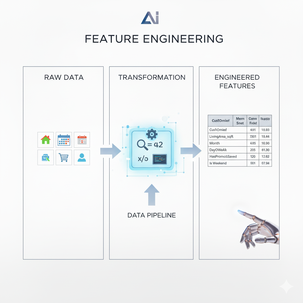
In the dazzling world of machine learning, it’s easy to become captivated by the latest neural network architectures or powerful gradient-boosting frameworks. However, even the most sophisticated algorithm is fundamentally constrained by the quality of the data it consumes. This is where the true art and science of Feature Engineering comes into play. Feature Engineering is the process of using domain knowledge to transform raw data into informative features that make machine learning algorithms work better. It is the crucial alchemy that turns base data into predictive gold.

While automated feature generation tools exist, the human-driven, creative process of Feature Engineering often yields the most significant performance gains. A well-engineered feature can unveil hidden patterns that a model might otherwise miss, leading to smarter, more robust, and more interpretable models. This article details seven powerful Feature Engineering tricks that will elevate your models from merely functional to truly intelligent.

1. Target Encoding: Informed Categorical Representation

The Problem in Detail:
Traditional methods for handling categorical variables, like Label Encoding (arbitrary numbers) and One-Hot Encoding (creating dummy variables), have significant flaws with high-cardinality data (categories with many unique values). Label Encoding Feature Engineering imposes a false ordinal relationship (e.g., implying ‘London’ < ‘New York’ < ‘Tokyo’), while One-Hot Encoding creates a “curse of dimensionality,” leading to sparse, high-dimensional data that can cause overfitting and computational bottlenecks.

The Technical Solution:
Target Encoding, also known as Mean Encoding, addresses this by replacing a categorical value with the average value of the target variable for that category. This directly injects predictive information into the feature itself.

Deep Dive & Implementation:

• Calculation: For a regression problem, the encoded value for a category is the mean of the target y for all training samples belonging to that category. For classification, it’s the probability of the positive class (P(y=1 | category)).
• Preventing Data Leakage: This is the most critical aspect. The encoding must be calculated only on the training data. The mapping from category to mean target value is then applied to the validation and test sets. A more robust method is using cross-validation within the training set to calculate the encodings, further reducing overfitting.
• Smoothing: To handle categories with Feature Engineering few samples and reduce noise, we can use smoothing. The encoding becomes a weighted average between the category mean and the global mean.
  Encoding = (n * category_mean + α * global_mean) / (n + α)
  where n is the sample count for the category and α is a smoothing parameter.

Example:
In a loan default prediction model, instead of one-hot encoding 500 different “Postal Codes,” we create a feature Postal_Code_Default_Rate. A postal code where 2% of historical applicants defaulted gets a value of 0.02. This tells the model directly about the risk associated with that location.

Why It Works:
It transforms a high-dimensional, uninformative representation into a single, highly predictive numerical feature. It allows linear models to Feature Engineering immediately understand the predictive power of a category without needing to split on it multiple times, as a tree would.

2. Polynomial Features: Modeling Interactions and Non-Linearity

The Problem in Detail:
Many real-world relationships are not linear. The effect of one feature often depends on the value of another. A simple linear model like y = β₀ + β₁x₁ + β₂x₂ cannot capture this interaction. It assumes the effect of x₁ on y is independent of the value of x₂.

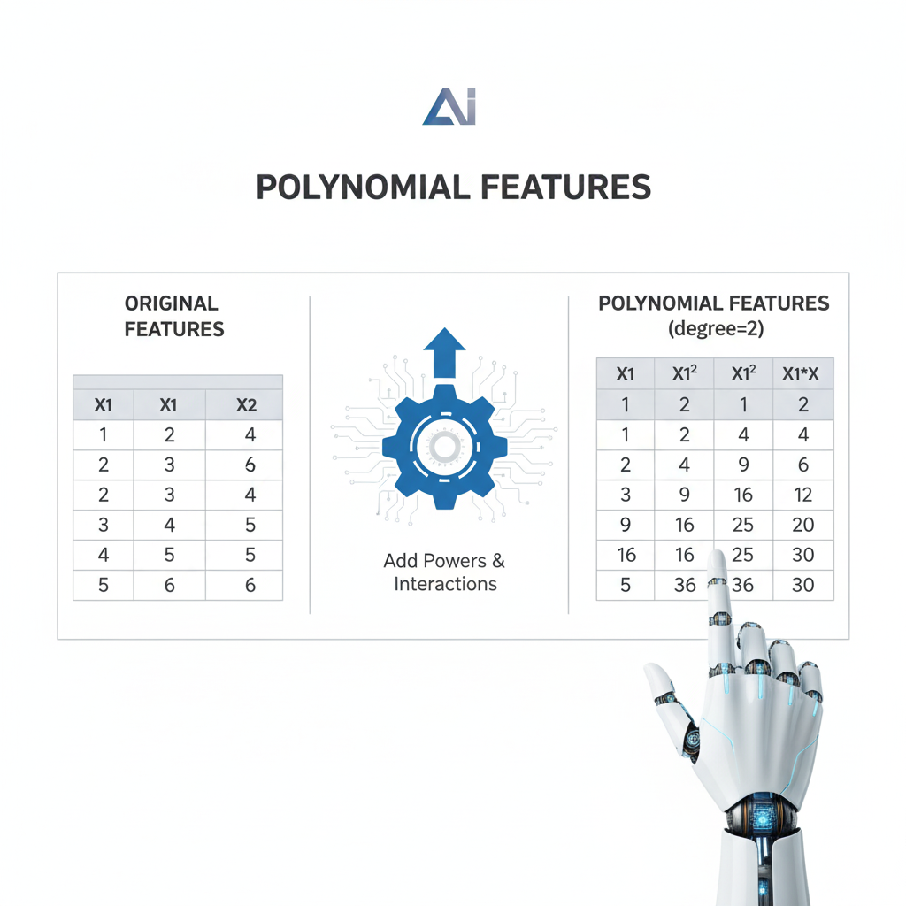
The Technical Solution:
Polynomial features explicitly create new features that are products (interactions) and powers of existing features, allowing the model to fit more complex, non-linear decision surfaces.

Deep Dive & Implementation:

• Interaction Terms: A feature x₃ = x₁ * x₂ allows the model to learn that the impact of x₁ changes depending on x₂. The coefficient for x₁ effectively becomes (β₁ + β₃x₂).
• Polynomial Terms: A feature x₁² captures quadratic relationships, allowing the model to represent U-shaped or inverted U-shaped curves.
• Degree Parameter: When using a library like sklearn.preprocessing.Polynomial Feature Engineering, the degree parameter controls the maximum power. A degree of 2 creates all interaction terms and squares; a degree of 3 also includes cubes and three-way interactions. Higher degrees exponentially increase the number of features and risk of overfitting.

Example:
In a real estate model, the value of an extra bedroom (x₁) is much higher for a large house (x₂ = high square footage) than for a small one. An interaction term x₃ = Bedrooms * Square_Footage allows the model to Feature Engineering capture this synergy. The model learns that the combined effect is more than the sum of its parts.

Why It Works:
It provides a structured way to introduce non-linearity into otherwise linear models. It makes the strong assumption of the linear model much more flexible, enabling it to approximate a wider range of underlying functions present in the data.

3. Binning / Discretization: Simplifying Complex Signals

The Problem in Detail:
Continuous variables can have complex, non-monotonic relationships with the target. For instance, the risk of a medical condition might be high for the very young and the very old, but low for middle-aged adults. Feature Engineering A linear model would try to fit a single straight line through this U-shaped relationship, resulting in poor performance.

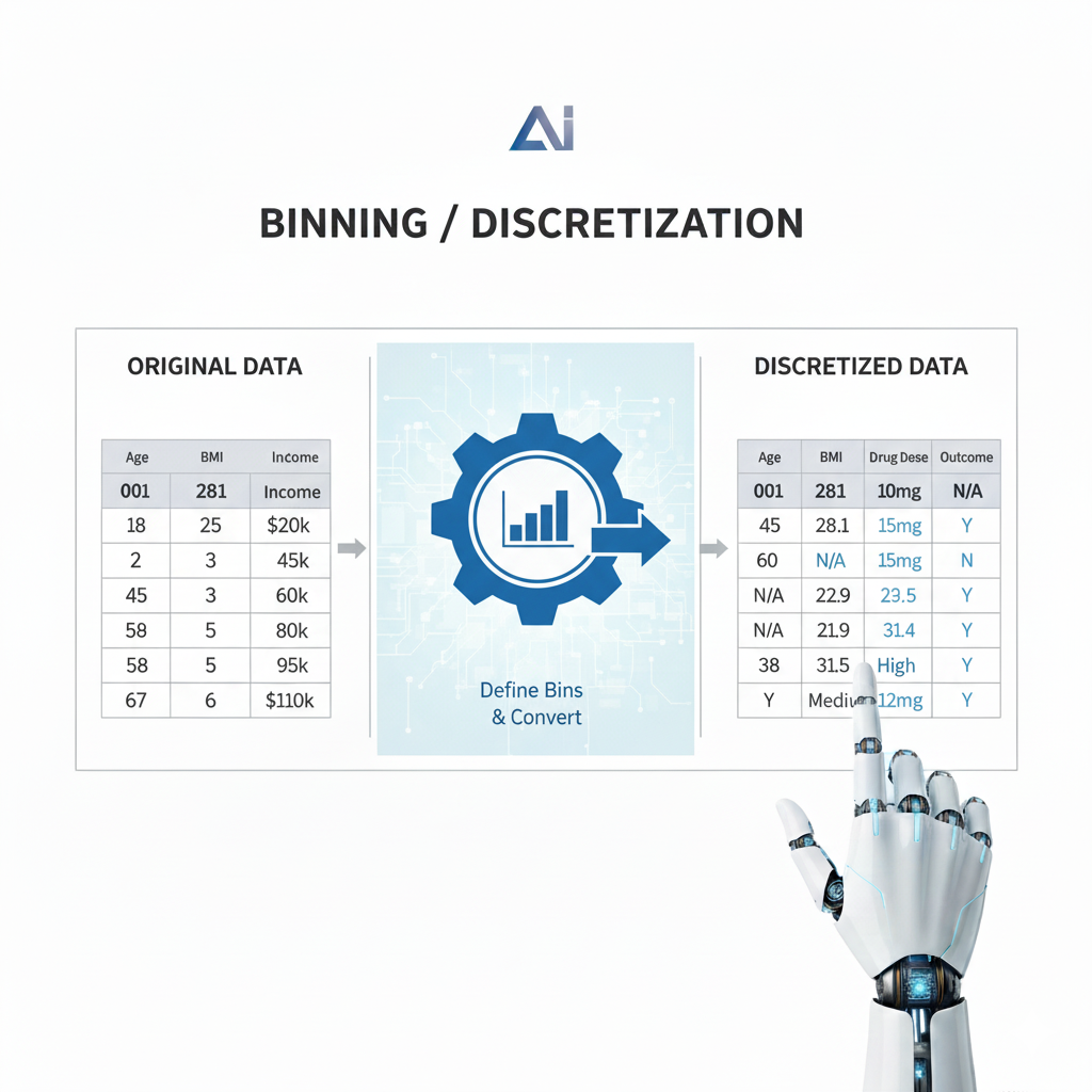
The Technical Solution:
Binning, or discretization, converts a continuous variable into an ordinal or categorical variable by grouping its values into intervals (bins). This allows the model to learn a separate “effect” for each range of values.

Deep Dive & Implementation:

• Methods:
  • Fixed-Width Binning: Divides the data into bins of equal width (e.g., age bins 0-10, 10-20, etc.). Simple but can create imbalanced bins.
  • Quantile Binning: Divides the data into bins such that each bin has approximately the same number of samples. Feature Engineering Creates balanced bins but the bin widths can vary significantly.
  • Domain-Knowledge Binning: Uses pre-defined, meaningful thresholds (e.g., BMI categories: Underweight, Normal, Overweight, Obese).
• Encoding: After binning, you can use ordinal encoding (if order matters) or one-hot encoding (if bins are truly categorical) for the new feature.

Example:
In a marketing model, converting “Annual Income” from a continuous value into bins like ["Low", "Medium", "High"] allows the model to learn that “High” income customers have a different propensity to purchase than “Low” income customers, without assuming a linear relationship where every dollar increase has the same effect.

Why It Works:
It reduces the noise and non-linearity of a continuous variable, making it easier for the model to learn. It is particularly effective for tree-based models, Feature Engineering as it simplifies the splits the tree has to make. It also handles outliers gracefully by placing them in the extreme bins.

4. Date/Time Decomposition: Unlocking Temporal Intelligence

The Problem in Detail:
A raw timestamp like 2025-03-15 14:30:00 is a single data point that contains a multitude of hidden, cyclical patterns. A model cannot natively extract the fact that this is a Saturday afternoon in March.

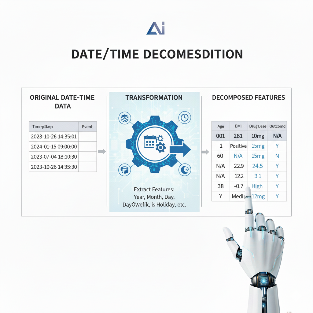
The Technical Solution:
Decompose the datetime object into its constituent temporal components, transforming a single, opaque feature into multiple Feature Engineering highly informative ones.

Deep Dive & Implementation:

• Basic Components: Extract Year, Month, Day, DayOfWeek, Hour, Minute.
• Cyclical Encoding: Time is cyclical—hour 23 is followed by hour 0. To represent this properly for a model, we use sine and cosine transformations.
  • Hour_sin = sin(2 * π * hour / 23)
  • Hour_cos = cos(2 * π * hour / 23)
    This places hours 23 and 0 close together in the new feature space.
• Domain-Specific Features:
  • Is_Weekend (Binary)
  • Is_Holiday (Binary, requires a holiday calendar)
  • PartOfDay (Categorical: ‘Morning’, ‘Afternoon’, ‘Evening’, ‘Night’)
  • Days_Since_Event (e.g., Days_Since_Last_Purchase)

Example:
For an electricity load forecasting model, the Hour_of_Day (cyclically encoded) and Is_Weekend are astronomically more predictive than the raw timestamp. The model can learn the daily cycle of human activity and the different pattern of weekends.

Why It Works:
It makes implicit temporal patterns explicit and digestible for the model. It transforms a single, complex feature into a set of simple, strongly predictive features that represent the seasonality, periodicity, and special events inherent in time-series data.

5. Cluster-Based Features: Adding Context through Proximity

The Problem in Detail:
Individual data points exist in a “feature space,” and their proximity to one another can be highly informative. A model might struggle to identify Feature Engineering that a group of customers with similar spending habits and demographics forms a distinct segment unless we explicitly point it out.

The Technical Solution:
Use unsupervised learning (clustering) to identify natural groupings in the data. Then, use the cluster assignments or distances to cluster Feature Engineering centers as new, high-level features for a downstream supervised model.

Deep Dive & Implementation:

1. Feature Selection: Choose the features relevant for clustering (e.g., for customer segmentation: Age, Income, Spending_Score). It’s often wise to scale these features first.
2. Clustering Algorithm: K-Means is a common choice. The number of clusters k is a hyperparameter.
3. Create New Features:
   • Cluster Label: Add the cluster ID as a new categorical feature (e.g., Customer_Segment = 2).
   • Distance Features: For each sample, calculate its distance to the centroid of each cluster. This creates k new numerical features that represent how “close” a sample is to each segment.

Example:
An e-commerce company clusters users based on Recency, Frequency, and Monetary value (RFM analysis). They find a “Champions” cluster (high F, high M) and a “At Risk” cluster (high R, low F). Adding the RFM_Cluster label to a churn prediction model gives it a powerful, pre-computed segment identifier, drastically improving its ability to target the “At Risk” group.

Why It Works:
It provides the supervised model with a “bird’s-eye view” of the data structure. It’s a form of automated, data-driven feature creation that summarizes complex multi-dimensional relationships into a simple, highly informative label or set of distances.

6. Advanced Text Feature Engineering: From Words to Meaning

The Problem in Detail:
Simple text representations like Bag-of-Words (BoW) create high-dimensional, sparse vectors that lose all word order and semantic meaning. They cannot understand Feature Engineering that “brilliant” and “excellent” are similar, or that “not good” is negative.

The Technical Solution:
Move from sparse, frequency-based representations to dense, semantic vector representations that capture meaning.

Deep Dive & Implementation:

• TF-IDF (Term Frequency-Inverse Document Frequency): An improvement over BoW. It weights words by how frequently they appear in a document (TF) but penalizes words that appear in many documents (IDF). This downweights common Feature Engineering but uninformative words like “the” or “and.”
• Word Embeddings (Word2Vec, GloVe): These are pre-trained models that map words to dense vectors (e.g., 300 dimensions) in a continuous space. Semantically similar words have similar vectors. To get a document vector, you can average the vectors of all words in the document.
• Sentence Transformers (e.g., from BERT): The modern state-of-the-art. These models are specifically designed to generate semantically rich vector representations for entire sentences or paragraphs. They are context-aware, meaning they understand that “bank” has a different meaning in “river bank” vs. “investment bank.”

Example:
For a movie review sentiment classifier, using a Sentence Transformer to convert the review text “A stunning and captivating performance, though the plot was weak” into a 384-dimensional vector will capture the mixed sentiment and overall meaning far more effectively than a TF-IDF vector that just counts words.

Why It Works:
These methods bridge the gap between human language and machine understanding. By representing text in a dense, semantic space, we allow our models to perform algebra on concepts, Feature Engineering leading to vastly better generalization on NLP tasks like classification, search, and translation.

7. Strategic Missing Data Handling: Treating Absence as Information

The Problem in Detail:
Missing data is often not random. The reason a value is missing can be informative. Simply using mean/median imputation erases this information and can distort the relationships between variables, introducing bias.

The Technical Solution:
Explicitly model the missingness. Instead of just filling the gap, create new features that indicate whether a value was missing and use more sophisticated imputation methods.

Deep Dive & Implementation:

• Missingness Indicator: For every feature with missing values, create a new binary feature: 1 if the original value was missing, 0 if it was present. This captures the potential signal in the pattern of missing data.
• Advanced Imputation:
  • For Numerical Features: Use KNNImputer or IterativeImputer (MICE). These methods model the feature with missing values as a function of other features, providing a more accurate and realistic estimate than a simple statistic.
  • For Categorical Features: The best practice is often to treat “Missing” as a new, valid category.

Example:
In a loan application, if the “Number_of_Credit_Cards” field is missing, it might be because the applicant has never had one (a signal of thin credit history)Feature Engineering. A Is_Num_Credit_Cards_Missing indicator would be a powerful feature. Meanwhile, the actual value could be imputed as 0, reflecting this likely reality.

Why It Works:
This approach acknowledges that “missingness” is a real-world event with potential causes. It preserves the informational value of the absence itself while providing a more principled and accurate guess for the missing value, leading to a more robust and truthful dataset.

Conclusion: The Strategic Imperative of Feature Engineering in the Modern ML Workflow

The journey through these seven powerful techniques reveals a fundamental truth: Feature Engineering is not a mere preliminary step in the machine learning pipeline; it is the continuous, intellectual core of the model development process. It represents the critical translation layer between the raw, unstructured reality of data and the structured, mathematical world of machine learning algorithms. While this guide has provided a deep toolkit—from the predictive efficiency of Target Encoding to the semantic richness of Sentence Transformers—their true power is only unlocked when applied not as isolated tricks, but as interconnected components of a strategic philosophy.

This philosophy is built on three pillars:

1. Intentionality over Automation: The most significant performance gains rarely come from blindly applying every technique in sequence. They come from a hypothesis-driven approach. Before creating a feature, ask: “What specific pattern or relationship is my current model likely missing, and what feature would explicitly provide that signal?” The choice to create polynomial Feature Engineering should be driven by a suspicion of interaction effects, just as the decision to use binning should be motivated by observed non-linearities. This thoughtful, diagnostic process is what separates a true data scientist from a technician.
2. Domain Knowledge as the Guiding Compass: The most elegant feature engineering solutions are often born from domain expertise, not just statistical insight. Knowing that a “weekend” effect exists in your industry makes datetime decomposition valuable. Understanding that a missing value in a medical test has a specific clinical meaning (e.g., “test was not deemed necessary”) informs a smarter missing data strategy. The synergy of subject-matter expertise and technical skill is where the most impactful features are conceived.
3. Iteration as a Discipline: Feature engineering is inherently iterative. It is a dialogue with your model. You create a new set of features, train a model, analyze its errors, and hypothesize why it failed. This analysis directly informs the next cycle of feature creation. This loop of Create -> Train -> Diagnose -> Refine is the engine of model improvement. The features that ultimately drive value are often discovered through this process of guided experimentation, not conceived in the initial blueprint.

The Future of Feature Engineering: Collaboration with AI

Looking ahead, the role of the data scientist in Feature Engineering is evolving, not becoming obsolete. We are entering an era of collaborative intelligence, where automated feature generation tools (like feature stores and AutoFE platforms) will handle the repetitive, scalable aspects of feature creation and management. However, the human role will become more elevated and strategic. The future data scientist will act as a conductor of an intelligent feature orchestra, focusing their efforts on:

• Curating and guiding automated systems, ensuring the generated features are logically sound and domain-appropriate.
• Designing the foundational blueprints and feature “primitives” that automated systems can combine.
• Interpreting complex feature interactions and ensuring model fairness and explainability, a task that remains deeply human-centric.

In conclusion, mastering Feature Engineering is to understand that data is not a static artifact to be mined, but a malleable substance to be shaped. The quality of your features determines the ceiling of your model’s performance. By embracing the mindset of a craftsman—thoughtful, iterative, and deeply knowledgeable—you empower yourself to build models that do not just find patterns in the data you have, but truly understand the complex reality you seek to model. The algorithms provide the engine, but it is the features that build the road. Your ability to engineer that road will forever be the defining factor between a model that is computationally clever and one that is genuinely intelligent.